



What is passive RF geolocation?
The expanding use of small unmanned aerial systems for inspection, agriculture, mapping, and military operations increases the need for reliable airspace awareness. Understanding what is present and how it is moving helps operators recognize unexpected activity before it becomes a safety or security incident. Radar and cooperative tracking provide important information, but small radar cross-sections, line-of-sight limitations, and platforms that do not report their position can leave gaps in detection and tracking.
Passive RF geolocation can complement these methods by locating transmitters through their existing radio emissions. Receivers observe signals such as control messages, telemetry, and video downlinks, then compare measurements to estimate the source’s position. The sensing system does not need to transmit an interrogation signal or receive a position report from the source. Processing these measurements in real time helps maintain a current picture as platforms move.
The signal being measured determines which transmitter is located. A control uplink may originate at a ground controller, while telemetry or video may originate on the aircraft. These links also have different propagation characteristics and signal bandwidths. Carrier frequency affects how a signal propagates and is received, while wider signal bandwidth generally supports more precise arrival-time estimation.
Time difference of arrival (TDOA) uses the difference in arrival time of the same signal at spatially separated receivers with known locations. Those differences reflect the distances the signal travels to each receiver. To extract useful location information, the system must distinguish propagation delay from differences in the receivers’ own time bases. A relative clock offset can bias the measured delay and shift the resulting location estimate. Receiver synchronization, signal bandwidth, and array geometry therefore need to be considered together when evaluating TDOA geolocation accuracy.
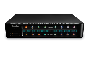
These requirements guide the choice of acquisition hardware. Moku:Delta combines eight synchronized inputs with up to 2 GHz bandwidth per channel, a blended clock architecture, and GNSS-referenced timestamping. Together, these capabilities support observing multiple RF bands while preserving timing information for comparison across receiver sites. The following sections explain how signal capture, receiver timing, and geometry affect the resulting geolocation measurement.
How time difference of arrival enables geolocation
Consider an RF transmitter at an unknown position and two receivers at known locations. If the transmitter is closer to one receiver, its signal reaches that receiver first. Time difference of arrival measures this relative delay. The transmitter’s emission time does not need to be known because it is common to both arrival times and cancels when they are subtracted.
Define the arrival-time difference as:
For direct propagation at approximately the speed of light, the corresponding difference in path length is:
Here, t₁ and t₂ are the arrival times at receivers 1 and 2, r₁ and r₂ are their distances from the transmitter, and c is the speed of light. This relationship assumes that relative receiver timing offsets and receive-chain delays have been accounted for.
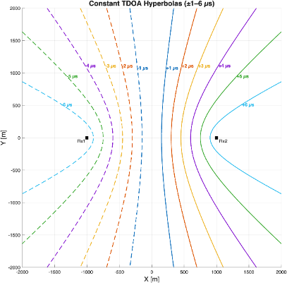
With this sign convention, a positive Δt means the signal arrives at receiver 2 first, so the transmitter is closer to receiver 2. A negative Δt means receiver 1 receives it first.
A single receiver pair provides a location constraint rather than a complete position estimate. In a two-dimensional model, the possible transmitter positions for a fixed nonzero range difference lie on one branch of a hyperbola. The magnitude of the delay defines the range difference, while its sign selects the branch. Many positions along that curve satisfy the same measurement.
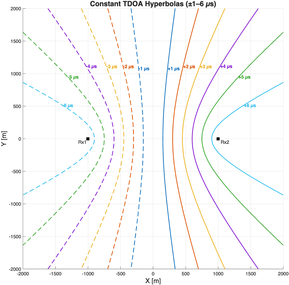
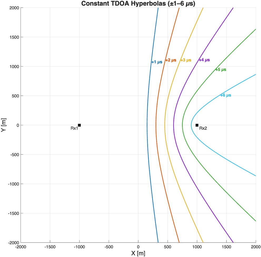
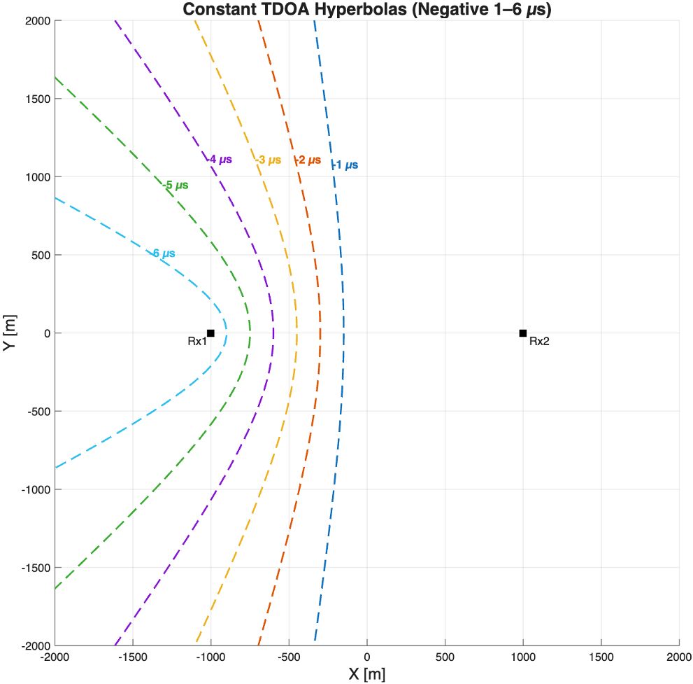
Adding a third receiver provides another independent arrival-time difference and another location constraint. Their intersection narrows the possible source locations. Three receivers are the minimum for this two-dimensional model, but they do not guarantee a unique solution for every geometry. Additional receivers or constraints may be needed to resolve ambiguity.
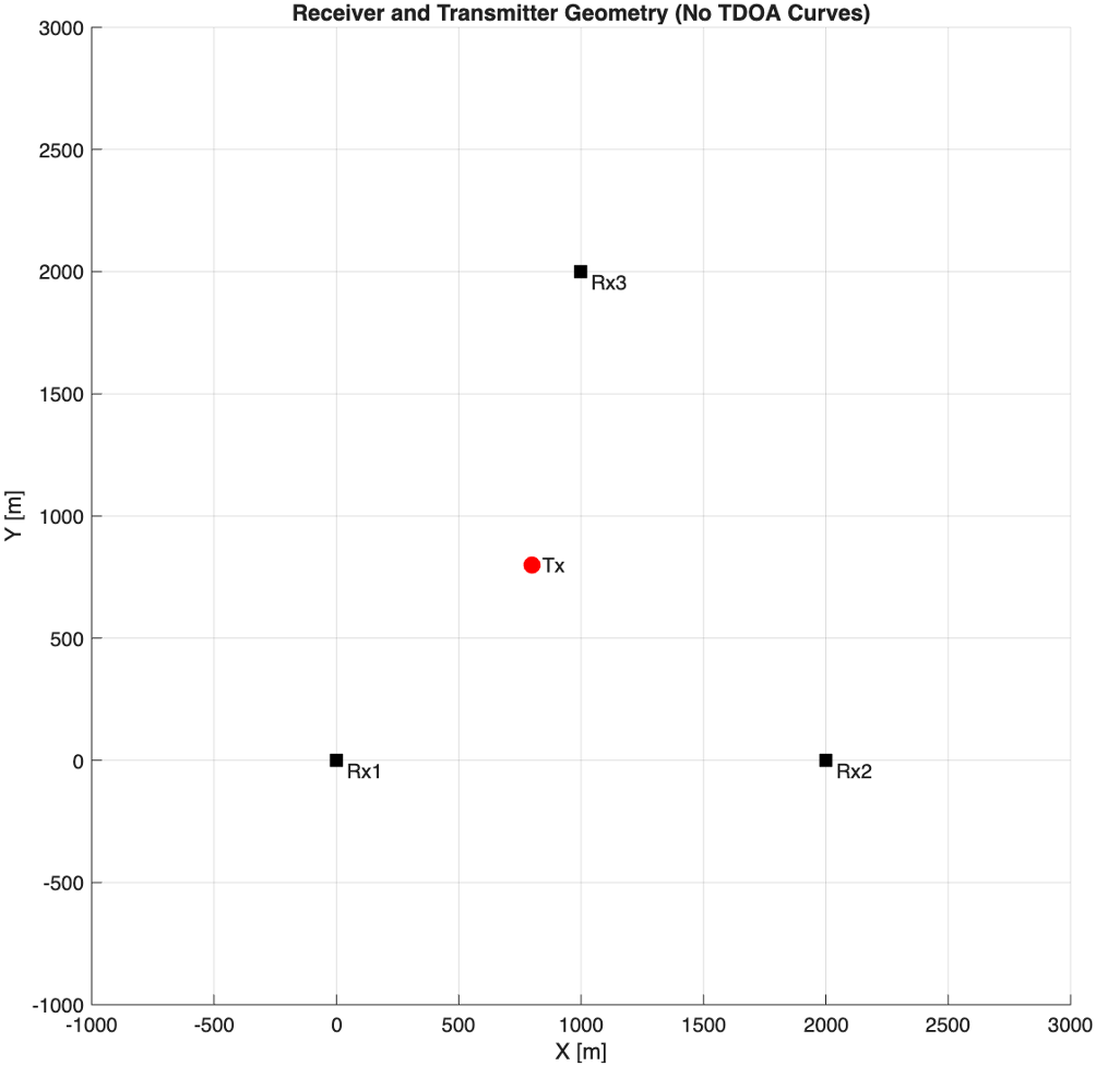
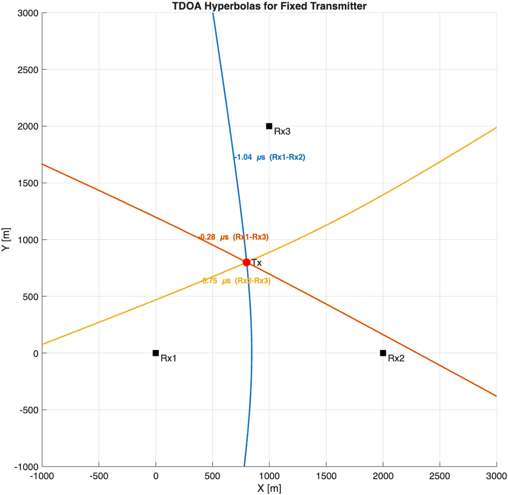
In practice, measurement errors can prevent the curves from intersecting at a single point. Position estimators, such as least squares or grid search, use the measurements to find a position that best fits the observed delays. The resulting accuracy depends on both the uncertainty in those delays and the receiver layout.
How timing synchronization affects TDOA accuracy
Each TDOA measurement defines a location constraint. An error in the measured delay shifts that constraint and changes the estimated transmitter position. Even small timing errors can produce substantial position errors, particularly when receiver geometry amplifies their effect. Accurate, stable timing across the receiver network is therefore essential for reliable TDOA geolocation.
Translating timing error into range difference
Using c ≈ 3 × 10⁸ m/s, the magnitude of a delay error translates into a range-difference error according to:
| Error in measured TDOA | Corresponding range-difference error |
| 10 ns | 約3メートル |
| 50 ns | 約15メートル |
| 100 ns | 約30メートル |
| 1μs | 約300m |
A 100 ns TDOA error corresponds to approximately 30 m of range-difference error. The resulting position error depends on how that constraint intersects the measurements from other receiver pairs. The conversion alone does not establish geolocation accuracy.
How receiver geometry affects accuracy
When TDOA curves intersect at well-separated angles, small shifts in the curves produce relatively small changes in the estimated position. At shallow intersection angles, the same shifts can produce much larger position errors. This sensitivity to receiver layout and transmitter position is described by geometric dilution of precision (GDOP). Favorable geometry constrains the location more tightly for a given measurement uncertainty.
Figure 6: Location uncertainty for an assumed 50 ns timing error. The uncertainty ellipse extends farther where TDOA curves intersect at shallow angles, illustrating how receiver geometry affects position uncertainty.
The same timing uncertainty can therefore produce different position uncertainty across the coverage area. Receiver placement should account for both signal reception and favorable geometry throughout the area of interest.
Moku:Delta GNSS-referenced timing and timestamped data give engineers greater flexibility to optimize this placement. Establishing a common time reference at each site reduces the need for dedicated timing connections between receivers. Each site still needs suitable GNSS reception, and the relative timing accuracy between systems must support the required geolocation accuracy.
Additional receivers can provide useful constraints, but their number alone does not determine accuracy. Receiver geometry and timing performance must be evaluated together. The next step is to identify where timing errors enter the measurement, starting with the receiver clocks.
Why TDOA receivers need to be synchronized
Even if a signal reaches two receivers at the same physical instant, a relative clock offset can make their recorded arrival times differ. That offset appears in the TDOA measurement as an apparent propagation delay. The receiver clocks therefore contribute directly to the accuracy of the measurement.
The receivers therefore need time bases whose relative offsets are known and controlled to the accuracy required by the application.
Figure 7: Location estimates with 1 µs synchronization error on Rx2. Errors will the amplified by geometric dilution of precision (GDOP).
The example figure introduces a 1 µs timing offset at one receiver. This adds approximately 300 m of range-difference bias and shifts the corresponding hyperbola. Improving the correlation or position estimator alone does not remove this offset; the timing relationship between receivers must be established separately.
Clock offset and drift
Clock synchronization must address both the initial time offset between receivers and their relative drift. If the clocks run at different rates, their offset changes over time. An alignment established at the start of a recording can therefore become less accurate as the recording continues.
A simplified model separates the contributions to the measured delay:
Measured TDOA = propagation TDOA + relative clock offset + relative receive-chain delay + delay-estimation error
The relative terms use receiver 1 minus receiver 2, consistent with Δt = t₁ − t₂. Cables and filters introduce delays before the signal reaches the measurement point. Differences between these receive chains can bias TDOA even when the clocks are aligned.
However, stable receive-chain delays and fixed clock offsets can be measured and corrected through calibration. But relative clock drift causes the offset to change after that correction is established. One of the easiest ways to ensure a stable timing relationship between receivers is to prevent clock drift from the other receivers in the first place.
How bandwidth and sample rate affect TDOA accuracy
Aligned receiver clocks make arrival times comparable, but the system still has to estimate the delay between the received signals. Cross-correlation is a common approach: recordings from two receivers are compared over a range of time shifts, and the location of the correlation peak provides an estimate of their relative delay.
How signal bandwidth affects the delay estimate
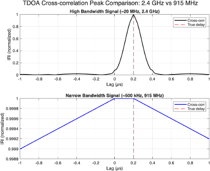
The shape of the correlation peak affects how precisely its location can be estimated. A signal with greater effective bandwidth generally produces a narrower peak, making small differences in delay easier to distinguish. A narrowband signal tends to produce a broader peak, so noise can make its location more difficult to determine.
The approximate 1/B relationship describes the scale of correlation-peak width, where B is signal bandwidth. Actual delay-estimation uncertainty also depends on signal-to-noise ratio, waveform structure, and the estimator.
How receiver bandwidth affects signal capture
Receiver bandwidth determines how much spectrum can be observed at once. The receiver must capture the signal bandwidth needed for the measurement, but wide instantaneous bandwidth offers another advantage when the signal’s frequency or transmission time is unknown.
A scanning receiver observes different frequency ranges in sequence. It can search a broad spectrum, but a short transmission may occur while the receiver is tuned elsewhere. Frequency-hopping signals introduce a similar challenge: the transmitter may leave a frequency before the receiver observes it. Whether the signal is captured depends on the scan timing, observation bandwidth, and transmission behavior.
A staring receiver continuously observes a selected frequency range. With sufficient instantaneous bandwidth, it can capture activity across that range without retuning between individual channels. For TDOA, this increases the opportunity for receivers at different sites to record corresponding bursts or hops. Those shared observations provide the data needed for cross-correlation.
Wideband recordings can also contain several signals of interest. Processing can separate them into frequency channels and correlate corresponding signals across receiver sites. This supports multiple delay measurements, provided the signals can be distinguished and the recordings retain a known timing relationship.
Moku:Delta’s eight synchronized analog inputs, each with 2 GHz bandwidth, allow different frequency bands to be acquired simultaneously. Suitable external filters and preamplifiers can optimize reception in each band, while downconverters translate higher-frequency signals into the inputs’ acquisition range. With one 2 GHz band mapped to each input, this configuration offers up to 16 GHz of aggregate spectral coverage.
Simultaneous acquisition reduces the risk of missing short transmissions or frequency hops while a scanning receiver is tuned elsewhere. The channels share a timing basis, but delays introduced by their separate signal paths still need to be characterized and calibrated for accurate TDOA measurements.
These acquisition capabilities preserve the available signal information. A wider receiver bandwidth does not, by itself, sharpen the correlation peak of a narrowband transmission; the delay estimate still depends on the captured signal and the processing applied to it.
How sample rate affects the delay estimate
The sample rate determines the spacing of the recorded samples:
Tₛ = 1/fₛ
A correlation evaluated at integer sample shifts has a delay grid with this spacing. Interpolation or other sub-sample methods can refine the peak location between grid points. The sample interval therefore sets the discrete grid, rather than an absolute limit on timing accuracy.
At 1 MSa/s, adjacent samples are 1 µs apart. A correlation evaluated only at integer sample shifts therefore has a delay grid with 1 µs spacing. A true delay between those grid points cannot be represented exactly by that estimate.
How GPS and GNSS time synchronization support TDOA receivers
GNSS provides a way for geographically separated receivers to relate their measurements to a common time reference without a physical timing connection. GPS, one of the global navigation satellite systems, broadcasts timing information that a timing receiver can use to compare or align a local clock.
For TDOA, that reference must be connected to the captured RF data. The workflow needs to preserve when the samples were acquired so that recordings from different receivers can be compared before their arrival-time differences are used to estimate position.
Establishing a common time reference
A GNSS timing receiver can provide a one-pulse-per-second (1PPS) output aligned to a reference second. Associated time information identifies the second to which that pulse corresponds. The acquisition system must use this information to establish a relationship between its local time base and the reference.
The pulse does not, by itself, describe when every RF sample was acquired. That relationship depends on the timestamp and sample-clock architecture. Some systems also discipline an oscillator from the reference to control clock rate.
Relating timestamps to captured samples
A common time reference must have a known relationship to the recorded samples. A timestamp identifies the time associated with an event or part of a recording, while the sample clock determines the spacing between samples. This relationship allows recordings from different receivers to be aligned on a common timeline.
For example, if a timestamp identifies the first sample of a block and the sample spacing is accurately known, the acquisition times of subsequent samples can be calculated. The timestamp and the data need to remain associated as the recording is exported or streamed into analysis software.
The receiver recordings can then be placed on a common timeline, their overlapping observations selected, and the signals compared by cross-correlation. Position estimation follows using the resulting delay measurements and known receiver coordinates. Clock-rate differences and uncorrected acquisition delays still need to be accounted for over the observation interval.
Timing accuracy and calibration
Timestamp resolution is the smallest time increment that can be represented. Timing accuracy describes how closely the timestamp corresponds to the actual acquisition time on the stated reference time scale. For TDOA, the relative timing error between receivers is particularly important. A finely resolved timestamp does not establish equally accurate alignment between devices.
GNSS timing also depends on installation and calibration. Propagation effects, multipath, and hardware delays contribute to the reference uncertainty. Within the RF acquisition path, differences in cable and filter delays can bias the arrival-time measurement even when receiver clocks are aligned. An FPGA-based acquisition architecture may help manage deterministic timing, buffering, and synchronization. The timing assessment must cover the path from the reference to the samples and the signal path to the measurement point.
Example: Timing limits in TDOA passive geolocation
Small UAS can use several RF links, including control, telemetry, and video downlinks. These provide different opportunities for passive geolocation. A 2.4 GHz control link, a 5.8 GHz video downlink, and a narrowband 900 MHz telemetry link can have substantially different signal bandwidths and transmission patterns. The signal selected for measurement therefore affects how precisely its arrival-time difference can be estimated.
Wider-band signals generally produce sharper correlation peaks, while narrowband signals make precise delay estimation more difficult. Observation time becomes another consideration when the available signal is transmitted in short bursts. A telemetry-radio example shows how these signal characteristics interact with sampling and integration time.
Figure 10: Moku:Delta Spectrum Analyzer observing real-time characteristics of the RFD900x telemetry radio compared with the common Frsky protocol using the 2.4 GHz ISM band
Consider a 900 MHz telemetry signal from an RFD900x-US radio. Each information channel occupies approximately 125 kHz, while the signal occupies an approximately 12.65 MHz span across its operation. The transmission is bursty, so the recording contains short periods of narrowband signal activity.
This gives the receiver a different measurement problem from a continuously available wideband signal. The narrow bandwidth of each burst produces a relatively broad correlation peak, and the selected observation window determines which bursts are available for the delay estimate. A longer window may provide more useful signal, but its benefit depends on the processing method and the stability of the measurement.
Resolving a delay between samples
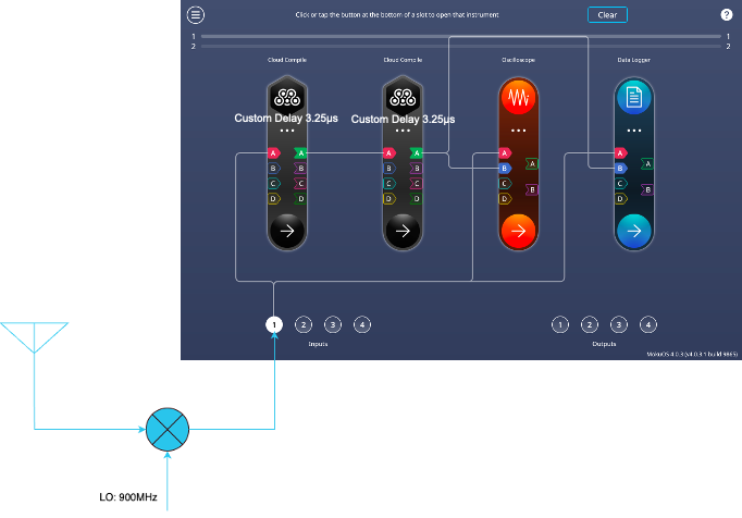
For the delay-estimation example, consider a 7 s recording sampled at 1 MSa/s, with a reference delay of 6.5 µs between the two receiver signals. The transmitter is assumed to remain stationary throughout the collection, allowing the effects of sampling and observation duration to be examined without introducing changes in delay from motion.
At this sample rate, adjacent samples are 1 µs apart. The 6.5 µs reference delay falls halfway between two integer sample shifts. An estimator restricted to those shifts can return 6 µs or 7 µs, but cannot represent 6.5 µs exactly.
Either nearest grid point is 0.5 µs from the reference delay. Even if the recordings were free of noise and perfectly aligned in time, choosing between those two integer shifts would leave this mismatch. It is a limitation of how the estimator represents delay, separate from clock synchronization.
Collecting more data does not add intermediate points to that grid. Interpolation or another sub-sample method is needed to represent a delay between them. Such a method can refine the estimate, but the available signal bandwidth and signal quality determine whether that refinement is accurate. A finely reported delay should therefore be validated against a known reference.
Comparing observation windows
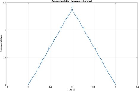
Timing error is a function of both bandwidth and data sampling rate. In this scenario, it is assumed that the TDOA between Rx1 and Rx2 is 6.5 µs. With a 7 second collection from RFD900x recorded at 1 MSa/s, the result is a “bursty” signal with a narrow bandwidth per burst.
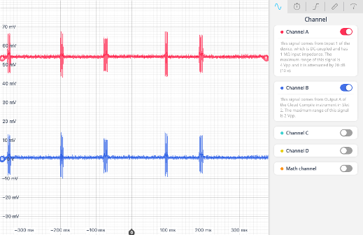
Assuming the transmitter is stationary for the full collection window, the TDOA estimate will be limited by the sampling resolution. Due to coarse sampling and limited bandwidth, the raw estimate may vary between 4 and 7 microseconds, depending on the integration window. A one and a half microsecond error equates to roughly 150 meters of position uncertainty. However, with a longer integration time of 100 ms or more, the correlation sharpens and the estimate converges back toward the true delay.
| Integration window | Delay estimate | Absolute error relative to 6.5 µs | Corresponding range-difference error |
| 10ミリ秒 | 4μs | 2.5μs | 約750メートル |
| 100ミリ秒 | 7μs | 0.5μs | 約150メートル |
| Greater than 1 s | 6μs | 0.5μs | 約150メートル |
The 10 ms estimate differs from the reference by 2.5 µs, more than the half-sample mismatch imposed by the nearest integer grid points. Sample spacing alone therefore does not explain that result. The selected signal interval and processing method also need to be examined; the available values do not establish the cause of the larger error.
A longer window can include more bursts and provide more information for correlation, but extending the observation does not necessarily resolve every source of error. Once the estimate reaches a neighboring integer lag, more data alone cannot represent the delay halfway between lags.
GNSS timestamping can help distributed receivers relate their measurements to a common time reference. Its benefit depends on the accuracy of the relative timing, the relationship between timestamps and captured samples, and calibration of hardware delays. Timestamp resolution alone does not establish equally accurate alignment between receivers.
Moku:Delta features for distributed passive RF sensing
A distributed passive RF system needs to capture the same transmission at multiple sites, preserve the timing relationship between recordings, and estimate their relative delay. Moku:Delta combines clock stability, GNSS-referenced timestamping, wide input bandwidth, and synchronized multichannel acquisition to address these requirements.
Clock stability throughout the observation
Moku:Delta’s clock-blending architecture combines local oscillators with GNSS referencing to support stability over different time scales. The local oscillators provide low short-term clock noise, while the GNSS reference corrects long-term drift. This helps maintain the timing relationship needed to interpret samples throughout an observation, rather than relying only on an initial clock alignment.
A common time reference across receiver sites
GNSS-referenced timestamps associate captured data with a common time basis, supporting comparison of recordings from geographically separated systems without a physical timing connection between sites. For TDOA, the timestamp-to-sample relationship and relative alignment accuracy must be established so that clock offsets can be distinguished from propagation delay.
Wide instantaneous bandwidth for intermittent signals
Moku:Delta provides up to 2 GHz analog bandwidth per input. Observing a broad frequency range simultaneously increases the opportunity to capture short bursts and frequency hops within that range. This is particularly useful when the transmission time or frequency is unknown: a scanning receiver may be tuned elsewhere during the interval needed for correlation.
Multiple bands observed simultaneously
Eight synchronized inputs allow separate channels to monitor different frequency bands. External filters, preamplifiers, and downconverters can adapt each receive path to its band of interest. With one externally downconverted 2 GHz band assigned to each input, the architecture can provide up to 16 GHz of aggregate spectral coverage, subject to the external front ends and acquisition configuration.
Together, these capabilities give engineers flexibility to select receiver locations and monitored bands while retaining a common timing basis. Signal-path calibration, suitable processing, and receiver geometry remain essential to translating those recordings into accurate position estimates.
結論
Passive RF geolocation can contribute to airspace awareness by locating transmitters through their existing emissions. For TDOA, the value of those observations depends on how reliably the receiver network measures the difference in arrival time.
Receiver timing, signal bandwidth, and geometry each affect the measurement in a different way. Clock offsets bias the delay, while limited signal bandwidth and an unsuitable estimator make it harder to resolve. Receiver instantaneous bandwidth also determines how much spectrum can be observed simultaneously: short bursts or frequency hops may be missed while a scanning receiver is tuned elsewhere, leaving no corresponding signal to correlate. Receiver geometry then determines how the remaining measurement error translates into position uncertainty.
GNSS-disciplined timing synchronization can provide a common time reference across receiver sites. Its benefit depends on the relationship between that reference and the captured samples, including calibration and clock stability over the observation interval. A practical TDOA design should therefore work back from the required position accuracy and update time, allocate the measurement uncertainties, and validate the complete acquisition and processing workflow against known conditions.
FAQ on TDOA timing and synchronization
While it is strongly recommended to maintain nanosecond-level timing synchronization (such as through GNSS synchronization or WhiteRabbit), there is no single timing-accuracy requirement for every TDOA system. It depends on the desired position accuracy, receiver geometry, and uncertainty in the delay estimate. Multiplying a timing error by the speed of light gives its equivalent range-difference error; for example, 10 ns corresponds to approximately 3 m. Position error then depends on how the measurements from the receiver network constrain the transmitter’s location. A synchronization specification should therefore be set as part of the complete error budget.
A relative clock offset adds a bias to the measured arrival-time difference. The position estimator can interpret that bias as a difference in propagation distance, shifting the inferred location. If the receiver clocks run at different rates, the offset changes during the observation interval. TDOA processing therefore needs both a known relative time alignment and sufficient stability over the period used for the measurement.
GNSS timestamping can support the alignment of recordings from geographically separated receivers, provided the timestamps have a known relationship to the acquired samples. It does not by itself determine the precision of the delay estimate or the accuracy of the resulting position. Signal bandwidth, SNR, sampling, processing, receiver geometry, and calibrated signal-path delays still contribute. The system’s performance needs to be established through an error budget and measurements under defined conditions.
Moku:Delta provides a reconfigurable platform for RF signal acquisition and processing. With the Gigabit Streamer, engineers can stream acquired data to external systems for recording and analysis, while Moku Compile supports custom FPGA processing before recording or playback.
Precision GNSS timestamping associates captured data with a common time reference, supporting the alignment of recordings from distributed receivers. These capabilities address the acquisition and timing stages of a TDOA workflow.
ソース
NIST。 One Way GNSS Time Transfer.
MathWorks。 Time-difference of arrival estimation.
MathWorks。 Object Tracking Using Time Difference of Arrival.
Liquid Instruments. ギガビットストリーマー.
Adamy, David L. EW 101: A First Course in Electronic Warfare.