


Stability measurements
Feedback loops, particularly in power electronics, need to be characterized in terms of their stability, which informs whether the system will behave as expected. Measuring loop behavior allows for stability assessment by looking at parameters such as frequency crossover, and gain- and phase- margin, so that loop-tuning parameters can be adjusted accordingly.
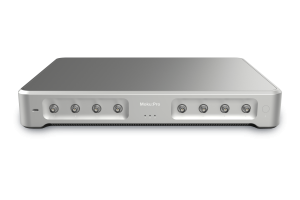
Stability is typically assessed by measuring loop gain and phase from a Bode plot using a Frequency Response Analyzer or a vector network analyzer. The Moku:Pro Frequency Response Analyzer can output up to four injection AC signals to Devices Under Test (DUTs) and simultaneously take in four response signals to plot gain and phase relative to the output injection signal.
The traditional and most straightforward way of measuring loop gain is by invasively breaking into the control loop circuit to inject a disturbance across an injection resistor in series with the feedback path. One side of the resistor connects to the feedback loop while the other side is connected to the response of the regulator. The ratio of these two voltages (output/input) can be analyzed in a Frequency Response Analyzer to measure the gain and phase margins for stability assessment.
The main drawback of this method is that the control loop circuit must be physically broken to insert an injection resistor. This is not always practical in situations where there may not be direct access to the loop such as fully enclosed systems like packaged ICs or very dense PCBs. Additionally, it is often not feasible to lift traces or add in components on an already designed and assembled device.
An alternative method to avoid physical loop interruption is to derive phase margins from the output impedance of the closed loop circuit. This method, coined Non-Invasive Stability Measurements (NISM), calculates the phase margin of a loop using the quality factor (Q), which is calculated from the magnitude and phase plots of the output impedance.
NISM methods – Second-order systems
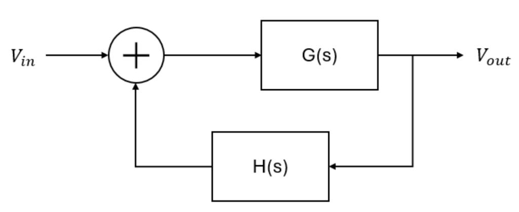
Control feedback loops are often modeled as second-order systems because their dynamics capture the most important aspects of system behavior, such as stability, damping, and transient response. Many real-world systems are technically of a higher order. However, their behavior is often dominated by a pair of complex-conjugate poles that are closer to the imaginary axis in the s-plane than all the other poles. These are called the dominant poles. In such cases, the system can be accurately approximated by a second-order model, making analysis easier without losing critical information about its overall behavior. Figure 1 shows a diagram for a generic control feedback system, where \(G(s)\) represents the transfer function of the plant and controller and \(H(s)\) represents the feedback transfer function. \(G(s)\) is defined in Equation 1. Using standard loop algebra, we obtain the closed-loop transfer function, shown as Equation 2.
\(G(s) = \frac{V_{out}}{V_{in}+V_{out}H(s)}\) (1)
\(\frac{V_{out}}{V_{in}} = \frac{G(s)}{1+H(s)G(s)}\) (2)
For a second-order system, Equation 1 can be expressed in terms of the standard canonical form shown in Equation 3 [1, Eq. (6.29)].
\(G(s) = \frac{\omega_n^2}{s(s+2 \zeta \omega)}\) (3)
where \(\omega_n\) is the natural frequency and \(\zeta \) is the damping ratio.
Assuming the feedback transfer function is equal to 1 (unity feedback), the closed-loop transfer function (Equation 2) becomes [1, Eq. (6.30)]:
\(T(s) = \frac{V_{out}}{V_{in}} = \frac{\omega^2_n}{s^2 + 2 \zeta \omega_n s + \omega_n^2}\) (4)
This is the standard transfer function equation for a second-order system. From this equation, we can calculate the quality factor, Q, which is a metric for how well the system resonates. First, we solve for the poles by applying the quadratic formula to the denominator of Equation 4, resulting in:
\(s = -\zeta \omega_n \pm j \omega_n \sqrt{1-\zeta^2}\)
The quality factor can then be calculated as:
\(Q = \frac{\omega}{2 \sigma}\)
where \(\omega\) is the oscillation angular frequency, or the imaginary part of the pole \((\omega_n \sqrt{1-\zeta^2})\), and σ is the decay rate of the oscillations, or the real part of the pole \((\zeta \omega_n)\). Plugging in the real and imaginary parts of Equation 5 into Equation 6, we obtain:
\(Q = \frac{\sqrt{1-\zeta^2}}{2 \zeta}\)
When \(\zeta \ll 1\),
\(Q \sim \frac{1}{2 \zeta}\)
While we now have a relationship between Q and the damping ratio, we can’t measure damping ratio of our system directly. We can, however, measure gain and phase of output impedance which can give us parameters such as group delay (\(\tau_g\)) which is the time delay of a signal envelope as it passes through a system. It is defined as the negative slope of phase response:
\(\tau_g(\omega) = \frac{d \phi (\omega)}{d \omega}\) (9)
where \(\phi (\omega)\) is phase in units of radians. At resonance, phase changes rapidly, so we expect to see a peak in the group delay signal at resonance, providing us with our resonant frequency and \(\tau_g\). Given that
\(\phi (\omega) = \arg{(T(j\omega))} = \arg{\left( \frac{\omega^2_n}{\omega^2_n – \omega^2 + j 2 \zeta \omega_n \omega} \right) } = -\arctan{\left( \frac{\omega_n \omega}{Q(\omega_n^2 – \omega^2)}\right)}\) (10)
at the resonant frequency, it can be mathematically proven that the group delay at resonance is equal to the inverse of the damping ratio times the natural frequency:
\(\tau_g(\omega) = -\frac{d \phi(\omega)}{d \omega} = \frac{1}{1+\left( \frac{\omega_n \omega}{Q(\omega_n^2 – \omega^2)}\right)}\left( \frac{\omega_n}{Q(\omega_n^2 – \omega^2)} + \frac{2 Q \omega_n \omega^2}{Q^2(\omega_n^2 – \omega^2)^2} \right)\)
\(= \frac{Q \omega_n (\omega_n^2 + \omega^2)}{Q^2(\omega_n^2 – \omega^2)^2 + \omega^2_n \omega^2}\)
\(\tau_g(\omega_n) = \frac{1}{\zeta \omega_n}\) (11)
To find the frequency \(\omega_{res}\) that minimizes denominator \(D\) of the magnitude of the transfer function \(T(j \omega)\), we take the derivative with respect to \(D\) and set it to zero:
\(|T(\omega)|^2 = \frac{\omega_n^4}{(\omega_n^2 – \omega^2)^2 + 4 \zeta^2 \omega_n^2 \omega^2}\) (12)
\(\frac{dD}{d \omega} = \frac{d}{d \omega}[(\omega_n^2 – \omega^2)^2 + 4 \zeta^2 \omega_n^2 \omega^2] = 0\) when \(\omega = \omega_{res}\) (13)
\(\omega_{res} = \omega_n \sqrt{1-2 \zeta^2} \approx \omega_n\) when \(\zeta \ll 1\) (14)
Substituting Equation 8 into Equation 11, we obtain a direct relationship between the quality factor, group delay, and resonant frequency:
\(Q = frac{|\tau_g(\omega_{res}) \ times \omega_n|}{2} = |\tau_g(f_{res}) \times f_{res} \times \pi|\) (15)
We can measure group delay and the resonant frequency from the gain and phase data using the Frequency Response analyzer to calculate Q. To calculate phase margin, we use the known relationship in Equation 13 [1, Eq. (6.31)]:
\(\phi_m = \arctan{\left( \frac{2 \zeta}{\sqrt{\sqrt{1+4 \zeta^4} -2 \zeta^2}} \right)}\) (16)
Substituting Equation 8 into Equation 16, we can calculate phase margin from Q:
\(\phi_m = \arctan{\sqrt{\frac{1+\sqrt{1+4Q^2}}{2Q^4}}}\) (17)
Using the gain and phase plots from the regulator’s measured output impedance, we can calculate the phase margin of the closed-loop system using Equations 15 and 17. Since output impedance can be measured without breaking open the control loop circuit, this is what enables non-invasive stability assessment.
Stability assessment
A control system’s stability is typically indicated by its gain and phase margins. Gain margin is how much the gain can be increased or decreased before instability occurs. On a Bode plot, as shown in Figure 2, it is the vertical distance between the magnitude curve and the 0 dB line (magnitude = 1), measured at the frequency where the phase equals -180˚.
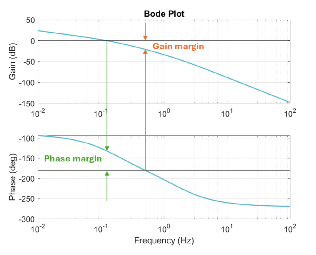
Phase margin indicates how far the system is from the point of instability in terms of phase. On a Bode plot it is the vertical distance from the phase curve to the phase value of -180˚ at the frequency where the magnitude is equal to 1 (or 0 dB), also known as the crossover frequency (see Figure 2). For stability, the phase margin must be positive. In practice, the required phase margin depends on the system design, but a commonly accepted minimum for adequate stability is around 30˚. As a rule of thumb, larger phase margins correspond to greater stability, though excessively large margins can reduce responsiveness which can be further evaluated by looking at crossover frequency.
In practical measurement contexts, such as NISM, output impedance is used to approximate phase margin but does not provide gain margin. Phase margin is typically the primary metric for stability assessment, as it directly gives information regarding the systems damping characteristics and gives us sufficient insight into transient performance—which is ultimately the key criterion for stability.
Experimental setup
Traditional stability measurement:
Figure 3 shows a diagram of the equipment setup to take traditional stability measurements. The device to be assessed is a voltage regulator board from Picotest (VRTS 1.5). The regulator board is powered by a DC power supply (7 VDC). At the top of the board, there are two Bode injection points across an injection resistor. The Moku Frequency Response Analyzer sends an AC signal out to an injection transformer (Picotest J2101A) to apply a sinusoidal perturbation signal across the injection resistor. The two inputs of the Frequency Response Analyzer are each connected to a Bode injection point, corresponding to prior- and post-injection responses.
The regulator board has three onboard switches that control two 100 μF capacitors and an output load resistor. One capacitor is aluminum electrolytic, and the other is tantalum. Because of the different capacitor materials, their equivalent series resistances (ESR) differ significantly. The aluminum electrolytic capacitor has a much higher ESR compared to the tantalum capacitor. The output load resistor was enabled for the traditional stability measurements to achieve a 25 mA load current and disabled for the NISM since the current injector already draws a 25 mA load current. Measurements were taken with each capacitor connected individually by enabling one while disabling the other. These measurements were taken for both the traditional and non-invasive stability measurements.
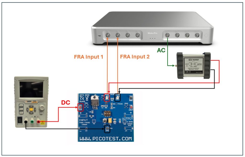
Figure 3: Traditional stability measurement system diagram. The Picotest VRTS 1.5 regulator board takes in 7 VDC at its input from the DC power supply. An AC signal from the Frequency Response Analyzer exits Moku:Pro from Output 1 and goes into the input of the injection transformer (Picotest J2101A). The perturbation signal on the output of the injection transformer gets injected onto the Bode injection points on the regulator board. Inputs 1 and 2 on Moku:Pro are each connected to one of the Bode injection points.
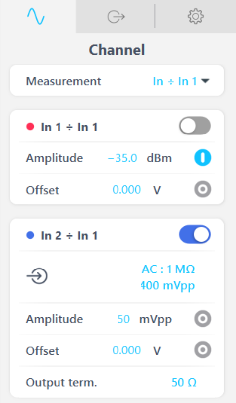
The settings for the Frequency Response Analyzer were configured as shown in Figure 4. The signal at Input 2 is divided by Input 1, plotting the voltage ratio from after the injection resistor to before. As the Frequency Response Analyzer injects the perturbation signal onto the injection resistor, it plots the gain and phase data across the same injection points. The amplitude is set to -35 dBm as higher amplitudes caused a non-linear response from the regulator and distorted gain and phase curves. The amplitude of the injection signal was therefore reduced until the response was no longer affected by the amplitude.
Non-invasive stability measurement
Figure 5 shows a diagram of the equipment setup to take non-invasive stability measurements. The same voltage regulator board is used and it is powered by the same DC power supply (7 VDC). The perturbation signal from Output 1 of the Frequency Response Analyzer is sent to the input of a current injector (Picotest J2111B), which is powered by a standard wall outlet voltage (120 VAC) through a regulated adapter (Picotest J2171A).
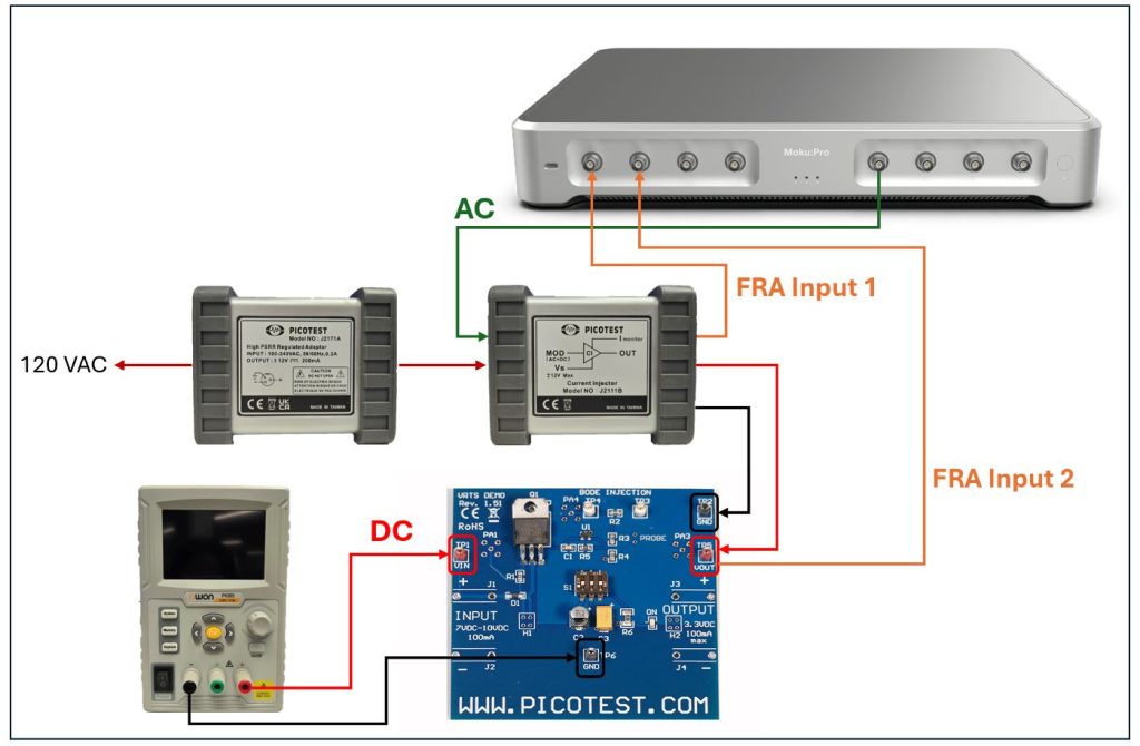
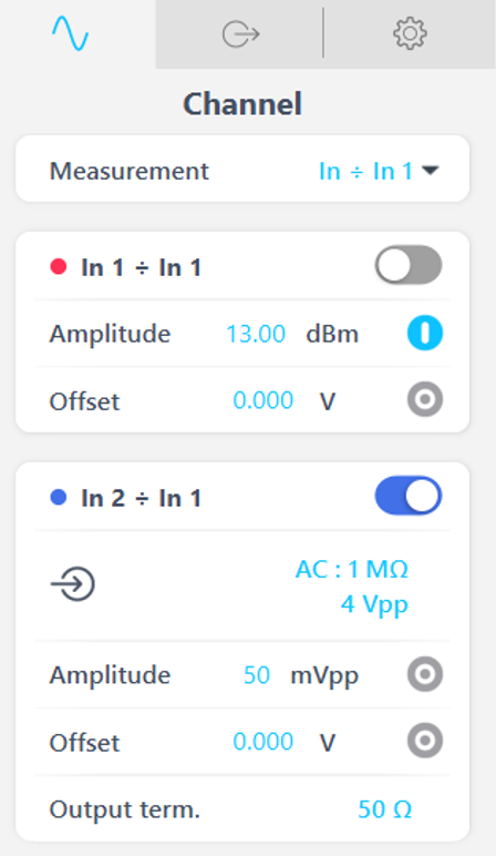
The output of the current injector is the perturbation signal which is connected to the output of the regulator board. The regulator output is also where the impedance is measured. The impedance is calculated by dividing the output voltage by the current on the output of the injector. To accomplish this measurement, Input 1 of the Frequency Response Analyzer is connected to the current and Input 2 is connected to the regulator output voltage. Figure 6 below shows the Frequency Response Analyzer settings to measure the regulator output impedance. The amplitude for NISM measurements is higher than the traditional method’s amplitude since the perturbation needs to be large enough to achieve a high enough SNR to accurately detect resonance from group delay.
Results
Figures 7 and 8 show the gain and phase plots for the traditional stability measurement setup (shown in Figure 3) with the tantalum and aluminum electrolytic capacitors enabled, respectively. Each plot was exported from the Frequency Response Analyzer in the Moku app as a matfile and plotted in MATLAB.
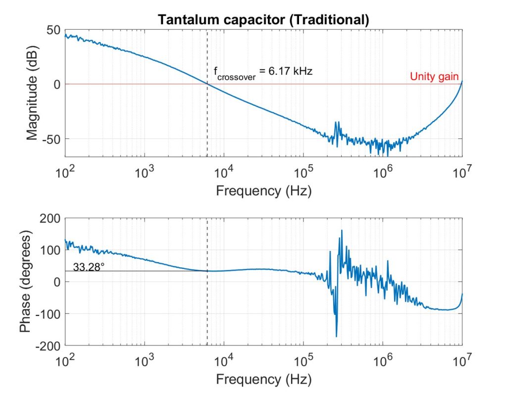
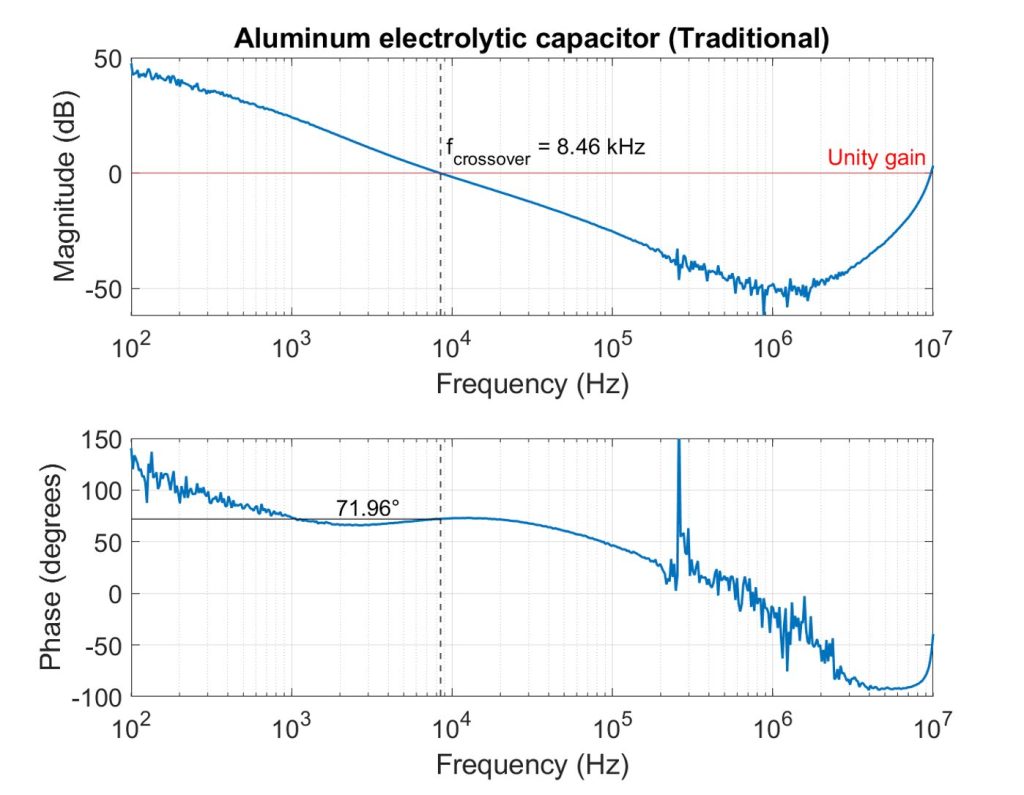
In each plot, we determine phase margin by finding the crossover frequency in the magnitude plot. This is the frequency at which the magnitude crosses the unity gain value (0 dB). The phase value at that crossover frequency is the phase margin.
The tantalum capacitor had a crossover frequency of 6.17 kHz and a corresponding phase margin of 33.28˚. The aluminum electrolytic capacitor had a higher frequency crossover at 8.46 kHz, resulting in a higher 71.96˚ phase margin. The higher ESR of the aluminum electrolytic capacitor shifted the zero caused by the ESR to a lower frequency, effectively adding phase lead before the gain crossover. This also reduced the slope of the magnitude response and allowed the loop to cross unity gain at a higher frequency.
Figures 9 and 10 show the magnitude and phase responses of the control loop with the tantalum and aluminum electrolytic capacitors enabled, respectively. These measurements were performed non-invasively using the setup shown in Figure 5.
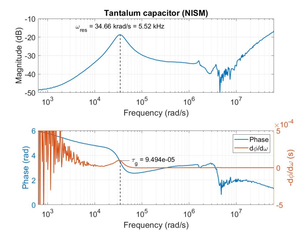
For Figure 9, there is a resonance peak at 5.52 kHz in the magnitude plot. For the phase data, group delay was calculated by taking the negative derivative of phase with respect to angular frequency and plotted to overlay the phase data. The peak in group delay occurs at the same frequency as the resonant peak, which makes sense since we expect phase changes to be more rapid around resonance. The group delay at resonance is 94.94 microseconds. Using these values for resonance frequency and group delay at resonance, quality factor is calculated to be 1.6454 from Equation 15. Plugging that quality factor value into Equation 17 gives a phase margin of approximately 33.67˚.
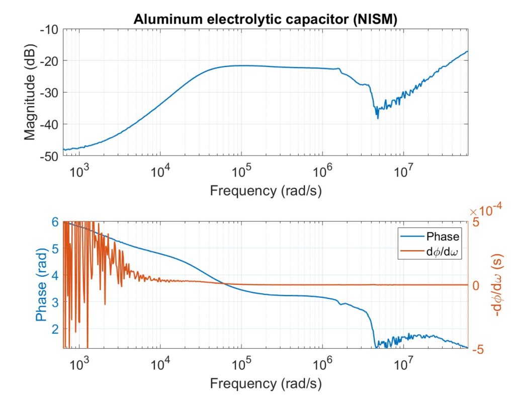
For the aluminum electrolytic capacitor, magnitude and group delay plots shown in Figure 10 do not exhibit a pronounced resonant peak. When this occurs, it indicates that the system is well-damped (approximately >70˚ phase margin) and is therefore stable. This assumption is made because the relationship between phase margin and damping ratio (shown in Equation 16), has a linear regime up until a certain phase margin value. This linear regime can be approximated as
\(\zeta \approx \frac{\phi_m}{100} \) (18)
The phase margin at which this regime becomes non-linear is the critical damping boundary and it is where the resonance peak disappears. If we find the local maximum of the magnitude of the second order transfer function (Equation 12) in the frequency domain, we get Equation 14. When set to 0, it equates to a damping ratio of 0.707. This value corresponds to a phase margin of roughly 70˚. Therefore, we assume that if there is no resonant peak, the phase margin is beyond approximately 70˚, indicating that the loop is well-damped and highly stable.
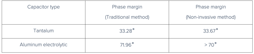
Table 1 shows a comparison of the phase margin values measured with each stability measurement method. There is overall great agreement between the values for each method. The phase margin obtained from the NISM with the tantalum capacitor was higher than the phase margin from traditional stability measurements by only 0.39˚. Since there was no clear resonance peak for the aluminum electrolytic capacitor in the NISM, we don’t have an exact value to compare with the phase margin from the traditional method. However, the assumed range from the lack of a resonance peak (>70˚) agrees with the 71.96˚ phase margin measured with the traditional method.
Summary
NISM is an effective method to assess loop stability without the need to physically break the circuit. In this application note, we used Moku:Pro’s Frequency Response Analyzer to compare the phase margin results obtained from traditional stability measurements with those derived from NISM, showing nearly identical values. Rather than requiring circuit interruption, NISM uses the circuit’s output impedance to determine the Q factor at resonance—based on the peak in group delay—and uses this relationship to reliably estimate phase margin.
We further evaluated the effect of capacitors with different ESRs on the regulator board. The results demonstrated that higher ESR values lead to increased phase margins, due to a shallower impedance slope and the resulting shift in gain frequency crossover.
Overall, NISM proves to be a reliable, efficient, and non-disruptive technique for analyzing control loop stability. The convenience of avoiding intrusive measurements makes it a valuable tool for both design verification and troubleshooting in power electronics. However, it does have some limitations to consider. NISM provides reliable estimations of loop stability within a limited phase margin range. While the traditional method requires breaking open the control loop, it enables a more comprehensive stability assessment that NISM cannot achieve. Therefore, for systems requiring analysis of larger phase margins, the traditional method is better suited. NISM is particularly advantageous for systems with smaller phase margins, and in environments where breaking open the loop is impractical or undesirable.
References
[1] G. F. Franklin, J. D. Powell, and A. Emami-Naeini, Feedback Control of Dynamic Systems, 8th ed., Global edition. Pearson, 2019.