Introduction
Classical and quantum light sources have broad uses, from quantum optics and quantum computing to classical fields such as laser interferometry. Light sources are often categorized by their statistical emission properties: whether they are coherent, thermal, chaotic, or quantum. Coherent light sources include lasers which have stable phases, and Poissonian fluctuations in the number of emitted photons. Thermal light sources, such as light bulb filaments or stars, produce light in bursts from large numbers of uncorrelated emitters. Quantum sources, such as squeezed light or single-photon emitters, exhibit ‘anti-bunching’ where the probability of detecting a photon immediately after you just saw one is lowest. This is an inherently quantum phenomenon that no classical light source can produce.
For quantum applications, it is often essential to characterize lights’ statistical emission properties to verify one has a genuinely quantum light source. Similarly, the accuracy of lasers should be limited by Poissonian statistics that govern the number of photons. One way to determine these statistical properties of light emission is through the \(g^{(2)}(\tau)\) correlation function, a widely used metric in classical and quantum optics.
In this application note, we present two methods to measure \(g^{(2)}(\tau)\) using Moku. As of MokuOS 4.1, the Time & Frequency Analyzer features a built-in \(g^{(2)}(\tau)\) calculator which operates in real time using a convolutional method. We can also use the Moku Time & Frequency Analyzer to capture and timestamp event data, then calculate \(g^{(2)}(\tau)\) in post-processing via a pairwise method. We outline both methods and verify them using Moku to simulate and record time-tagged photon events. We then walk through the procedure for generating a time-delay histogram and using it to calculate the second order correlation function. We then compare this to the Time & Frequency Analyzer’s built-in \(g^{(2)}(\tau)\) function.
What is the second-order correlation function?
The second-order correlation function, \(g^{(2)}(\tau)\), measures the fraction of events in a time interval τ relative to the average number of detected events over a span \(T\). The value at \(\tau=0\) is of particular importance, as this can infer information about how many concurrent photons are emitted by the light source. For example:
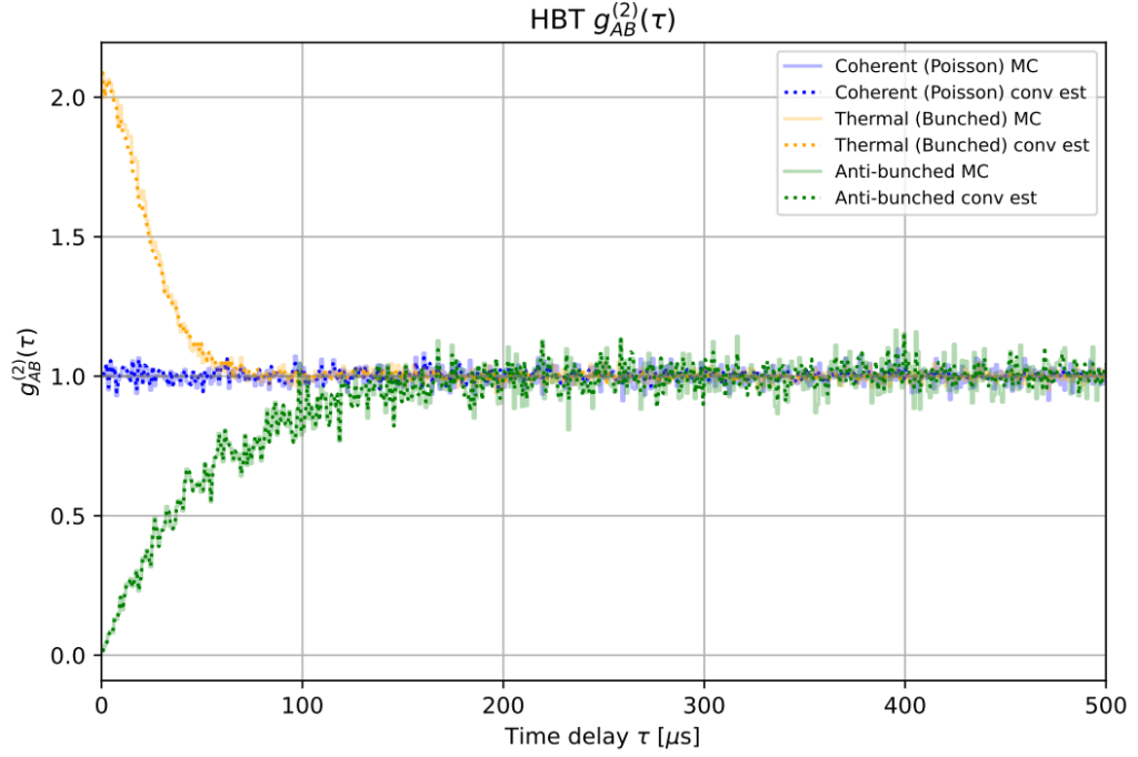
If \(g^{(2)}(0)>1\), then the light source tends to emit photons in groups. This is called bunching behavior and is usually indicative of a thermal light source. For example, \(g^{(2)}(\tau=0)=2\) means that there are twice as many events at time delays close to zero compared to the average number of events separated by any time delay \(\tau\) within some length of time \(T\).
If \(g^{(2)}(0)<1\), then the light source tends to emit photons at regular intervals, with very little chance of emitting more than one at a time. This is called antibunching behavior and is a desirable trait for single-photon sources.
If \(g^{(2)}(0)=1\), then there is no correlation between emitted photons. This is usually true of a coherent light source, such as a laser.
A simulation of these three cases can be seen in Fig. 1 below.
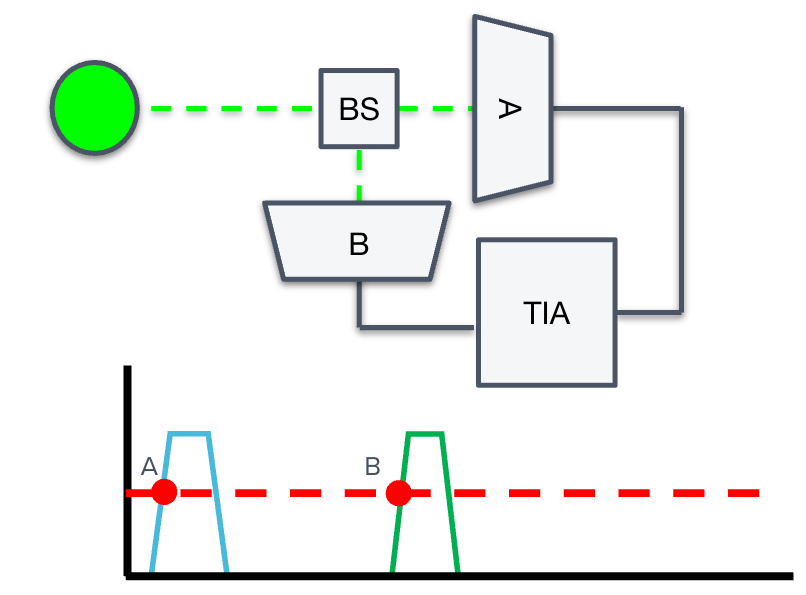
To demonstrate how to use and compute \(g^{(2)}(\tau)\), we introduce the Hanbury-Brown-Twiss (HBT) effect. In a HBT experiment (see Fig. 2), the source under test emits a stream of photons into a 50/50 beam splitter, which directs the individual photons to one of two optical paths. Two single-photon detectors (arbitrarily labeled “A” and “B”) monitor the arrival of photons traveling each of these arms. Any optical path difference between the two arms will result in a temporal offset between the arrival of photons at the two detectors. If a detector records a photon event, it generates an electrical pulse, which it passes to the time interval analyzer (TIA). The function of the TIA is to accurately timestamp and record photon events at both A and B, for later postprocessing. As we will derive in the next section, the time correlations between events A and B will determine the value of the second-order correlation function.
Quantifying the second order correlation function and coincidence rate
The second-order correlation function \(g^{(2)}(\tau)\) is given by the time-averaged product of photon detection counts:
\(g^{(2)}(\tau) = \frac{\langle n_A(t) n_B(t+\tau) \rangle}{ \langle n_A(t) n_B(t) \rangle} \)
where \(n_A(t)\) and \(n_B(t)\) are the rate of detected photon events at detectors A and B at times \(t\) and \(t + τ\), respectively. Quantities inside \(\langle . \rangle\) are time averages, i.e.,
\(\langle n_A(t) n_B(t+\tau) \rangle = \lim_{T\to\infty} \frac{1}{T}\int_0^T n_A(t) n_B(t+\tau) dt \).
Having established a quantitative definition of \(g^{(2)}(\tau)\), let now discuss how to determine \(\langle n_A(t) n_B(t+\tau) \rangle\). This is the time-averaged coincidence rate, or the probability density of finding a photon at time \(t\) and another at time \(t +\tau\), regardless of where the first event came from. This means that an initial event at A could be followed by a first, second, or third event at B in a cascade. All these events must be considered when calculating the coincidence rate. Then these τ values are binned and normalized to yield an estimate of \(\langle n_A(t) n_B(t+\tau) \rangle\).
Measuring the time delay histogram
A key part of HBT measurements is the time interval analyzer, which collects the photon events and generates a histogram of time intervals. The Moku Time & Frequency Analyzer can be configured to perform HBT measurements, as seen in Fig. 3. In this setup, single-photon detectors (SPDs) A and B are connected to Inputs A and B of Moku. The Time & Frequency Analyzer can be configured to detect the output pulses from the SPDs, with Input A acting as the “start” and Input B acting as the “stop.” For more details on how to configure the Moku for HBT measurement, refer to our configuration guide on the topic.
During the measurement sequence, the Time & Frequency Analyzer records the delay time between successive events A and B, from which a number-density of delays between pairs of detected photons is constructed in real time. It is important to note that the real-time histogram generated by the Time & Frequency Analyzer only measures first-step events and thus some post-processing is required to calculate \(g^{(2)}(\tau)\). Fortunately, there is a way to convert the distribution of time interval data into an approximation of \(g^{(2)}(\tau)\), through a process called self-convolution, discussed in the next section. This forms the basis for the on-board \(g^{(2)}(\tau)\) calculator in the Moku Time & Frequency Analyzer.
Analyzing the interval data
Assume a histogram of interval times captured by the Time & Frequency Analyzer. We call this distribution \(k(\tau)\), which records the time delay between each photon and the first subsequent photon in the other stream. In pseudo-code, we can imagine it written:
for A_time in A:
    find the first B_time after A_time
    tau = B_time - A_time
As we stated in the previous section, \(k(\tau)\) is a probability density function for first-step delays only. While \(k(\tau)\) ostensibly resembles \(\langle n_A(t) n_B(t+\tau) \rangle\), it only includes first-order contributions and excludes photons caused by longer cascades. For example, photons arriving at times \(t + \tau_1 + \tau_2\) or \(t + \tau_1 + \tau_2 + \tau_3\) are not considered.
For this reason, \(k(\tau)\) is not typically used to calculate \(g^{(2)}(\tau)\) directly. Instead, one must manually count each explicit coincidence between events A and B, up to some maximum time. In pseudo-code, the process is:
for A_time in A:
    find all B_time that occur after A_time, within some t_max
    for each B_time
        tau = B_time - A_time
These τ values are then binned to create a histogram and normalized appropriately so that \(g^{(2)}(\tau)=1\) represents no correlation at that delay. While direct and intuitive, this method scales poorly because one must compare every event A to every event B. This leads to \(O(N_A \times N_B)\) operations, which can quickly grow out of control if the rate of events is high. For this reason, this feature is difficult for hardware to implement in real time.
The Moku Time & Frequency Analyzer thus implements a second, alternative method to calculating \(g^{(2)}(\tau)\) in real time, one that is more conducive to the unique properties of an FPGA. This method involves performing higher-order self-convolutions of \(k(\tau)\), represented by the quantity \(k^{(n)}(\tau)\). Each \(k^{(n)}(\tau)\) describes the probability density that a photon occurs at time τ, given that it is the nth photon in a cascade. In other words, it corresponds to the delay distribution from the initial event to a descendant n photons later. The total probability density G(τ) of observing a photon at time τ after the initial trigger, regardless of which generation it came from, is proportional to the infinite sum [1]:
\(G(\tau) \propto \sum_{n=1} ^\infty k^{(n)}(\tau)\).
This sum should be interpreted as a logical OR over mutually exclusive paths, as it accounts for the probability that a photon appears at time τ due to the 1st generation, or the 2nd, or the 3rd, etc. Each term represents an independent possibility, and their sum gives the total arrival density at delay τ. Hence,
\(g^{(2)}(\tau) \propto G(\tau)\).
In the next section, we will measure \(g^{(2)}(\tau)\) two ways: one by recording the timestamps and calculating the full pairwise values, the second using the built-in calculator on Moku.
Experimentally verifying \(g^{(2)}(\tau)\) with the Moku Time & Frequency Analyzer
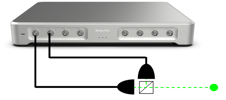
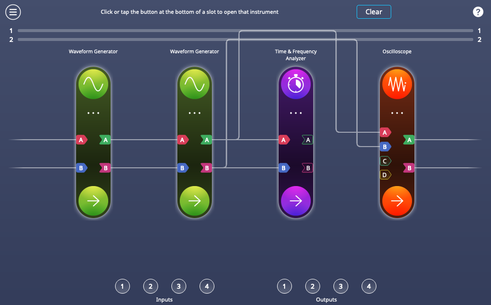
To simulate an Poissonian event distribution, we use an all-electrical setup with Moku:Pro. Making use of Multi-Instrument Mode, we partition the Moku FPGA into four instrument slots, each of which emulates part of the measurement. See Fig. 4 for details and connection map.
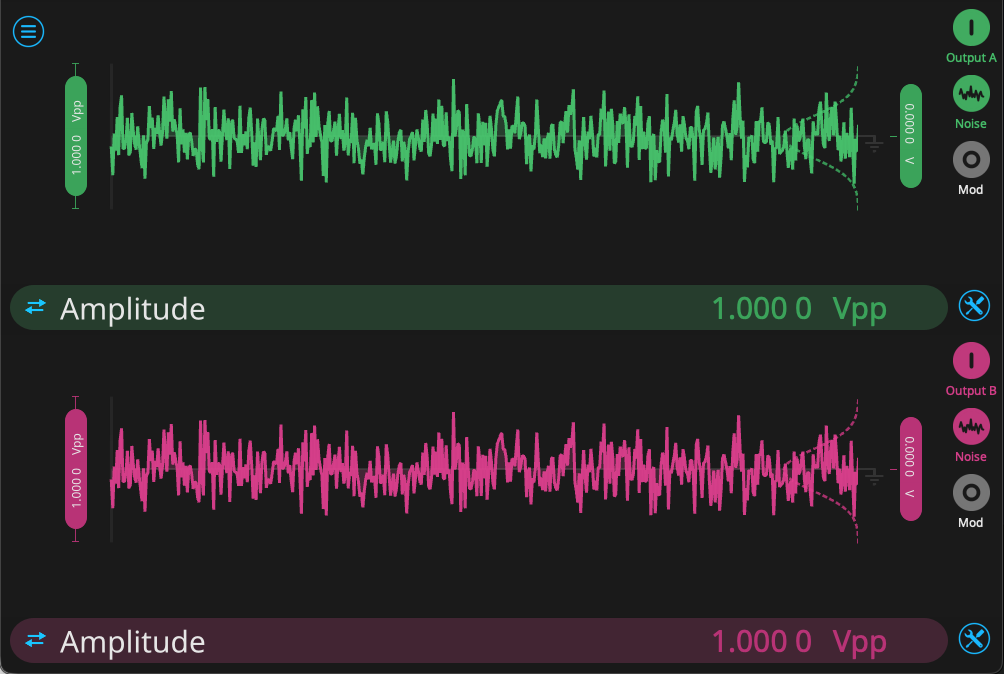
First, we configure the Waveform Generator, which will provide two uncorrelated streams of noise. From the configuration screen, we enable Output A and Output B. We select the “noise” function for both, and set the range to 1 V. See Fig. 5 for the Waveform Generator configuration.
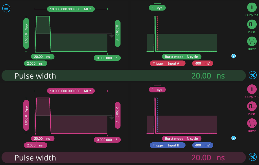
Second, we use another Waveform Generator to mimic the function of a pair of photodetectors. We select a pulse output with repetition rate of 10 MHz and a pulse length of 20 ns. We enable N cycle burst mode, with a threshold of 400 mV. Each channel is triggered by one of the noise sources on the first Waveform Generator. In this way, the second Waveform Generator will trigger when the input hits a certain voltage threshold, outputting a square pulse reminiscent of the behavior of a single-photon detector. In this case, the threshold is 400 mV, but one can alter this value to change the frequency of “photon” events. The configuration of the second Waveform Generator is seen in Fig. 6.
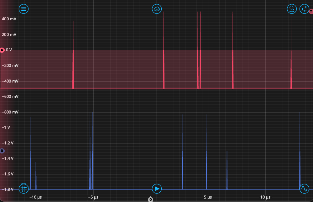
Third, we configure the Time & Frequency Analyzer to detect “photon” events occurring on Inputs A and B. From the Events tab, we set the event threshold to 0 V on a rising edge, and then measure the time interval beginning with Event A and ending with Event B. The repetition rate is high, so we can measure in Windowed Mode, with a measurement interval of 100 ms, which will capture a sufficient number of events. Finally, we set up the Oscilloscope in the fourth slot to observe the output. After setting up all instruments and enabling the output from the Waveform Generator, we see the output reflected on the Oscilloscope as in Fig. 7. Both channels A and B should have “event” pulses randomly distributed between them, sometimes in close time proximity.
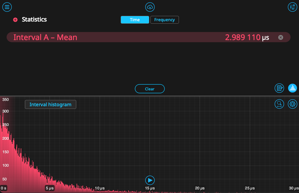
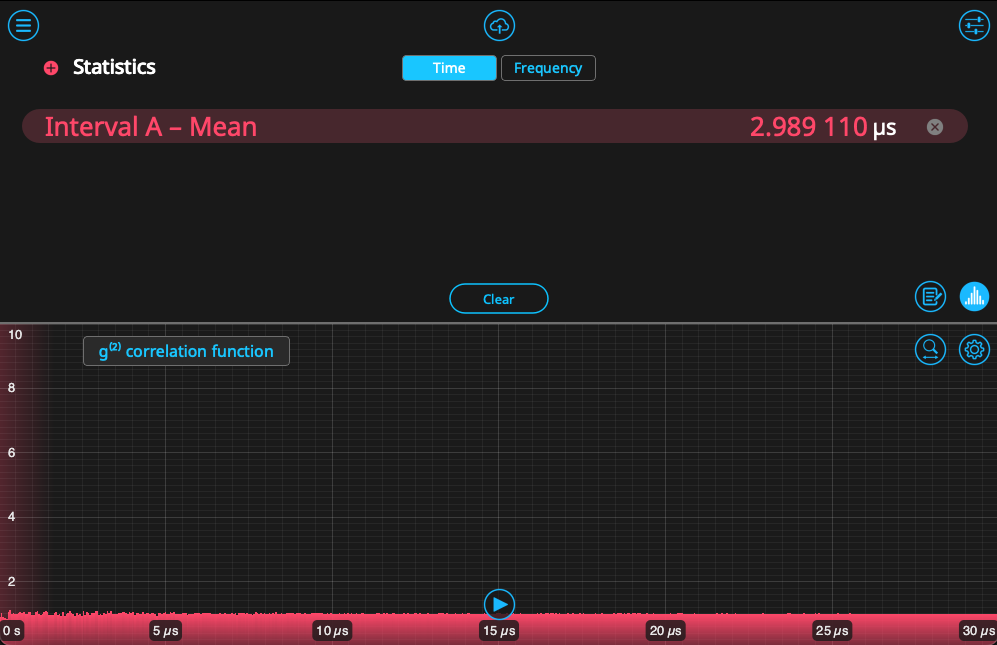
Returning the Time & Frequency Analyzer, we likewise start to see these events populate in a histogram. As established in the previous section, this histogram only reflects the time interval between nearest events and does not account for 2nd- or 3rd-order cascades. We can view the on-board calculation of \(g^{(2)}(\tau)\) by clicking on the button titled “Interval histogram,” which will switch the display. These can be seen side-by-side in Figure 8. Since the correlation is the result of self-convolution of the histogram, it looks substantially different. The values hover near 1, indicating that there is no correlation between Events A and B – the expected answer for a pseudo-random distribution.
To generate \(g^{(2)}(\tau)\) using the pairwise method, we can log the raw timestamp data to a host PC by disabling the histogram and clicking on the data logger icon in the bottom right. Set the start trigger and collection time, then click the red button to begin logging. After logging, click the cloud icon, then select the most recent data file. Make sure the format is set to “NumPy” format, then send it to your destination of choice. In the next section, we will use a Python script to calculate \(g^{(2)}(\tau)\).
Calculating \(g^{(2)} (\tau)\) with Python using timestamp data
In order to demonstrate the agreement between these methods, we will now use the timestamp data generated by the Time & Frequency Analyzer to estimate \(g^{(2)}(\tau)\). This Python notebook is available from our Github.
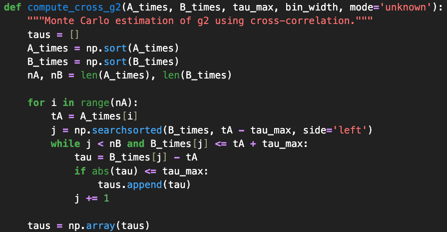
Our first step, after making standard package imports, is to import the data into two arrays, A_times and B_times. We then calculate the next occurring B event after an A event, giving us the first-order interval information – the same as plotted by the Moku Time & Frequency Analyzer. With both the time stamp and histogram information, we can perform the calculation of \(g^{(2)}(\tau)\) via the methods described in the previous section. The first method is seen in Fig. 9, where we search for every event in B_times that occurs after each event in A_times. These values are then binned and normalized appropriately.
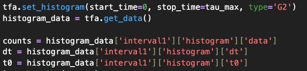
For the second method, the self-convolution of the first-order event histogram this gives us a quantity proportional to the time-averaged coincidence rate as defined earlier. We obtain this by setting up the Time & Frequency Analyzer and obtaining the histogram using the get_data() function, which returns the list of time bins and the correlation value calculated for each. The code can be seen in Fig. 10.
We now compare the two methods by plotting the full, pairwise calculation alongside the plot produced on board the Moku device. This comparison is seen in Figure 11. Both methods agree well, producing values of \(g^{(2)}(\tau)\) near 1 across the entire timespan, which is expected for two uncorrelated sources.
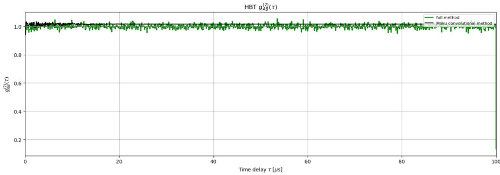
The convolutional and pairwise methods may show small differences in \(g^{(2)}(\tau)\), particularly near \(\tau \approx 0\), due to their different computational approaches. The convolutional method uses binned histogram data obtained by Moku, while the pairwise method explicitly evaluates all event pair combinations.
Both methods are mathematically valid approaches to computing second-order correlations. For most applications, the methods produce equivalent results. Users should be aware that edge cases or specific detector configurations may show minor differences between the two approaches.
Summary
The second-order correlation function is a powerful tool for evaluating the temporal dynamics of light sources and is crucial for quantum optics applications ranging from secure communication to photonic computation.
We have used the Moku Time & Frequency Analyzer to calculate the second-order correlation function, \(g^{(2)}(\tau)\), via two methods. In the first, we used the built-in calculator in the Moku Time & Frequency Analyzer to generate the function via a convolutional method. Secondly, we demonstrated how to capture high-resolution time-tagged photon events and analyze them with Python, calculating \(g^{(2)}(\tau)\) with a full pairwise method. We showed good agreement between these methods when plotted together.
Whether investigating coherent lasers or single-photon emitters, familiarity with both methods of calculating \(g^{(2)}(\tau)\) will enable users to measure deviations from ideal behavior and quantify source performance.
References
[1] Chen-How Huang, Yung-Hsiang Wen, and Yi-Wei Liu, “Measuring the second order correlation function and the coherence time using random phase modulation,” Opt. Express 24, 4278-4288 (2016).