The Nyquist sampling theorem
The Nyquist-Shannon sampling theorem relates a signal’s bandwidth to the sampling rate required to resolve it. If you have a sine wave of period T, you can reconstruct that wave if you sample at least two points within one period. For example, a signal of 1 MHz has a period of 1 us. You would need to take one sample at least every 500 ns, a rate of 2 MSa/s, to capture this sine wave. However, signals are often more complicated than simple sine waves. To reconstruct a multi-tone analog signal from digital samples, you need to capture at least two points within the period of the highest frequency component that exists in the signal.
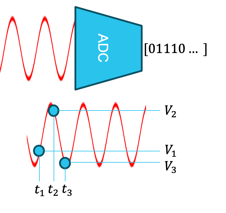
In the case of multiple input channels, the specified sampling rate can be per-channel rate or total combined rate. This depends on the nature of the analog-to-digital converter (ADC) as well as processing speed (see Figure 1). For example, Moku:Delta offers a sampling rate of 5 GSa/s on each of its eight input channels.
This leads us to the Nyquist-Shannon sampling theorem: to accurately capture a given signal, the sampling rate needs to be at least twice the bandwidth of that signal. This is laid out in Equation 1:
\(\frac{f_s}{2} > B\) (1)
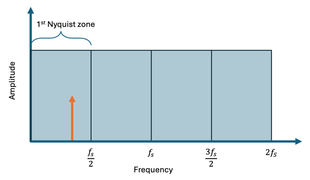
Where \(f_s\) is the sampling rate of the ADC and B is the bandwidth of the signal. Indeed, this frequency cutoff \(f_s/2\) represents the edge of the so-called first Nyquist zone. Subsequent Nyquist zones occur at integer multiples of \(f_s/2\), as seen in Equation 2:
nth Nyquist zone edge \(= \frac{nf_s}{2} \) for \(n= 1,2,3…\) (2)
For our example of 2 MSa/s our first Nyquist zone would range from 0 Hz to 1 MHz. The second Nyquist zone would then range from 1 MHz to 2 MHz. A diagram of different Nyquist zones is seen in Figure 2. In later sections we will discuss more about how signals in higher Nyquist zones impact measurements.
Aliasing
When the sample rate is below (slower than) 2x the frequency of the signal of interest, aliasing occurs. Usually, aliasing is a negative thing to be avoided, but in the case of undersampling, we use it to our advantage.
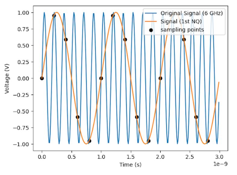
Even if a signal or frequency component lies outside the first Nyquist zone, the ADC will still digitize it. For frequencies above the Nyquist limit, the ADC will not sample enough points within the period to accurately capture the signal. The result is called aliasing. Like its name suggests, aliasing occurs when a higher frequency component seems to appear at different, lower frequency. We can illustrate an example of this behavior in Figure 3. The samples of the 6 GHz signal are also perfectly fit by a 1 GHz signal, which does lie within the first Nyquist zone. As a result, the ADC will interpret this as a frequency of 1 GHz. We say that the 6 GHz tone is “aliasing” to 1 GHz, as it is not a true 1 GHz tone but an artifact of undersampling by the ADC.
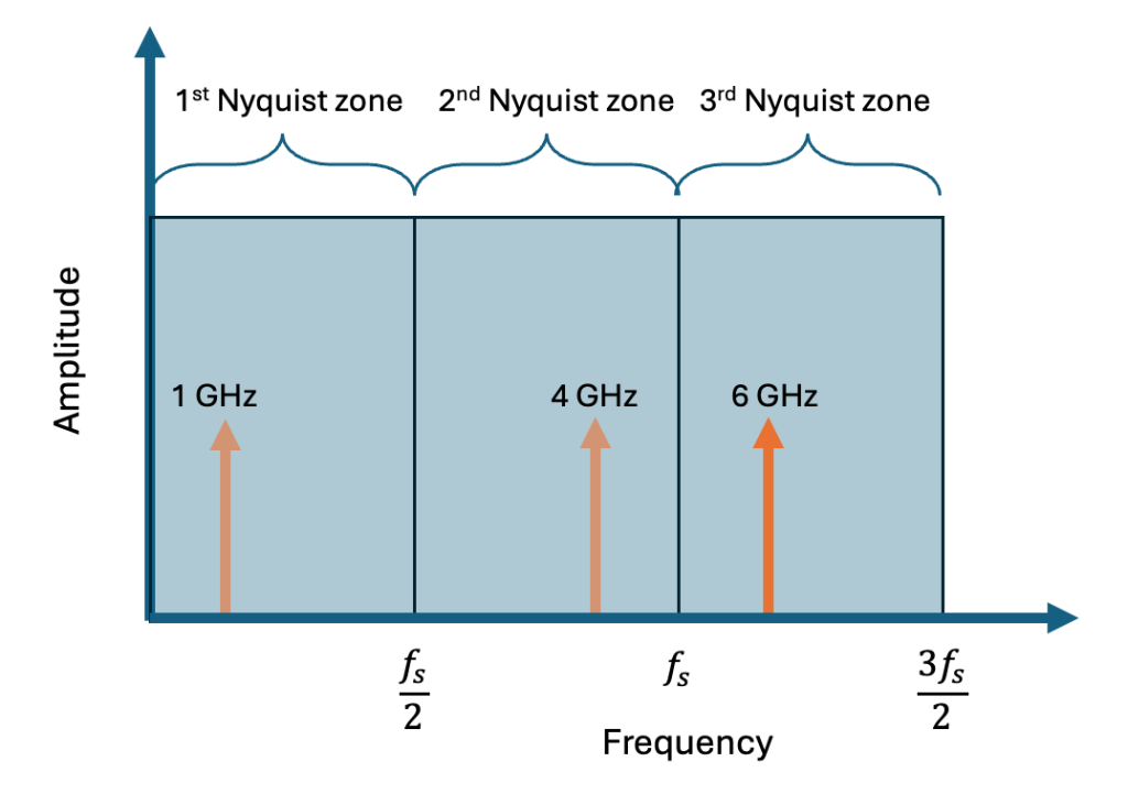
Undersampling causes high frequency signals to be folded into lower Nyquist zones at specific frequencies. If an incoming signal occurs in a higher Nyquist zone, then the alias of this signal will mirror around the Nyquist zone cutoff frequencies. For example, the 6 GHz signal is 1 GHz away from the Nyquist zone edge of 5 GHz, so the alias in 2nd Nyquist zone will occur at 4 GHz. This 4 GHz signal is 1.5 GHz away from the 1st Nyquist zone edge of 2.5 GHz, so the alias will occur at 1 GHz. This can be seen in both Figure 3 and Figure 4. When given a frequency in the first Nyquist zone f1, we can calculate which higher Nyquist zone frequencies will alias at f1 with Equation 3:
\(f = n f_s \pm f_1\) for \(n=1,2,3…\) (3)
Where fs is the sampling rate. The end result is this: due to aliasing, input frequencies of 6 GHz, 4 GHz, and 1 GHz all appear identical to the ADC.
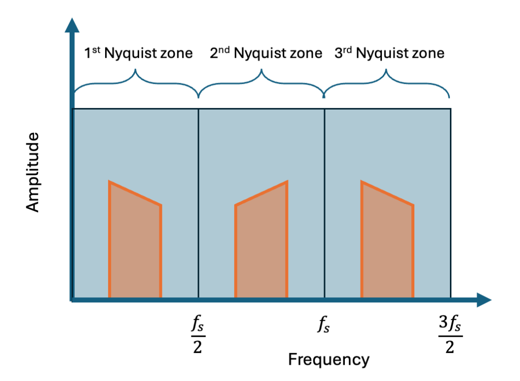
This behavior gives rise to so-called spectral mirroring. If an input signal consisting of a range of frequencies lies in the 3rd Nyquist zone, then the spectral profile of the signal will appear reversed in the 2nd Nyquist zones. The profile in the 1st Nyquist zone will look the same at the original. This can be seen in Figure 5.
Aliasing is generally inconvenient for the end user and best avoided. Aliasing by high frequency components present in a signal can significantly distort the measured spectrum at lower frequencies. To continue using our example, imagine a 1 GHz signal containing weak image components at 4 GHz and 6 GHz. These components are typically very low power, but they can still alias down to 1 GHz and make the base frequency appear to be higher power than it is.
This problem compounds for more complex or frequency-modulated signals. However, a simple solution exists. Most analog frontends have a filter stage before the signal passes to the ADC. Filtering appropriately will heavily reduce the effects of aliasing, giving it the name anti-aliasing filtering.
Using Moku:Delta and higher Nyquist zones
Moku:Delta has a sampling rate of 5 GSa/s and a stated bandwidth of 2 GHz. The frontend contains a lowpass filter which attenuates any input frequencies above 2 GHz. This cuts out high frequency components and accurately preserves the signal within the first Nyquist zone. However, with care on behalf of the end user, it is possible to detect higher frequency signals via undersampling.
With MokuOS 4.2 release Moku:Delta offers the option to route the input signal through a balun instead of the 2 GHz low-pass filter. This option can be found with other signal conditioning options when using single-instrument mode, or by clicking on the input port in Multi-Instrument Mode and can be enabled separately for each of the 8 inputs on Moku:Delta. This option is seen in Figure 6.
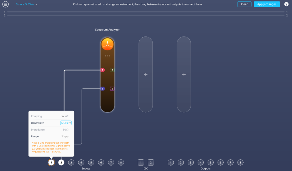
This feature allows users to access the full analog bandwidth of the Mokus:Delta’s ADCs, for viewing with various Moku instruments such as the Spectrum Analyzer or Lock-in Amplifier, or streaming data to storage with the Gigabit Streamer. Undersampling effectively acts as a mixer, downconverting signals at a specific frequency while preserving the phase information. When using this option, any stray frequencies, including noise, will also be folded into the first Nyquist zone.
In order to get the best results, you will need to understand the nature of your signal profile and consider the following:
Analog bandwidth
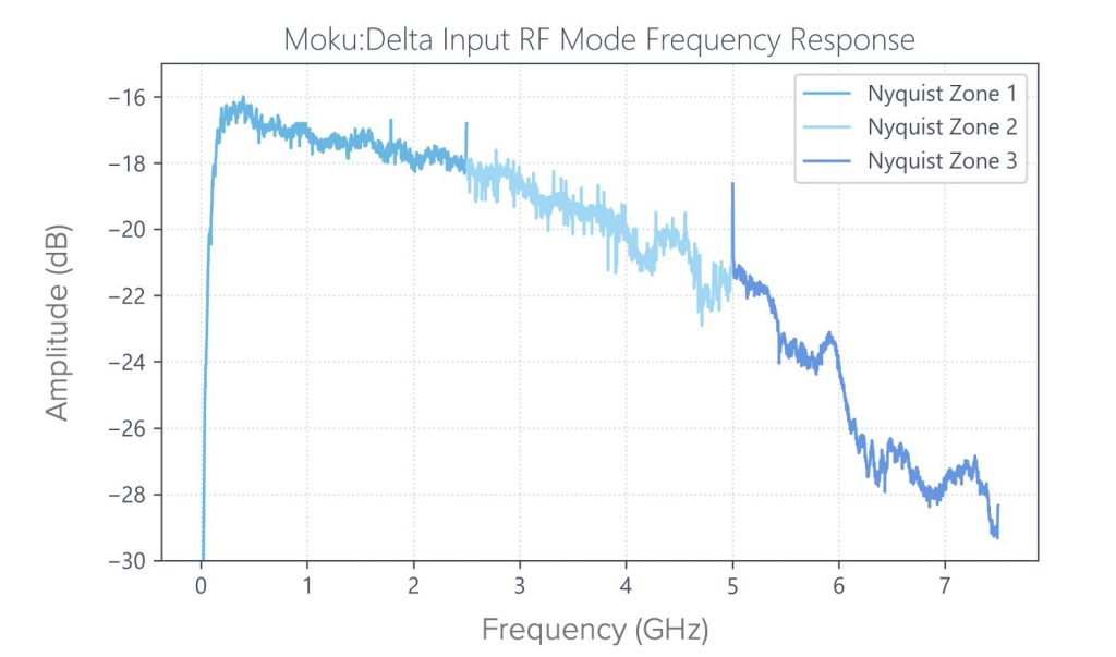
While undersampling can theoretically be used to look at signals in any Nyquist zone, the maximum usable frequency will be limited by the analog bandwidth of the Moku:Delta To give Moku:Delta users an estimate of the expected attenuation of high-frequency input signal, in Figure 7 below we provide the frequency response plot for the first three Nyquist zones (up to 7.5 GHz). Given the roll off in the 3rd Nyquist zone, the maximum recommended frequency for Moku:Delta with undersampling is 6 GHz. This also means that while undersampling can be useful for detecting spurs or harmonics, it is generally not suitable for absolute power measurements.
Filtering
To improve measurement of a signal of interest it is important to apply your own filtering. Adding a bandpass filter with an appropriate, narrow passband will reduce interference and noise. For example, if your signal of interest is around 4 GHz, then applying a bandpass filter or lowpass filter after signal generation will help to reduce the presence of other harmonics. In Delta’s case, the 4 GHz signal will alias 1 GHz, but other high frequency signals, such as those at 8 GHz, will be greatly reduced in amplitude and you will see a more accurate representation of the original signal. See the next two sections for examples.
Qubit state readout with the Lock-in Amplifier
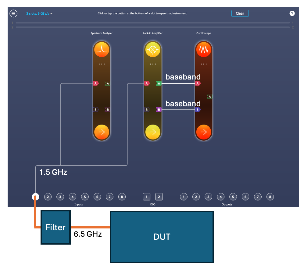
We use the following example to illustrate a use case for undersampling. In quantum computing, solid-state or superconducting qubits are typically measured via a technique called dispersive readout. A readout signal at 6.5 GHz is sent from an AWG and then is reflected off the qubit. The phase shift of this readout pulse contains information about the state of the qubit. In this case, the only signal of interest exists in a narrow band around 6.5 GHz, so undersampling can be an effective way to retrieve this information. The presence of this signal can be verified using the Moku:Delta Spectrum Analyzer, where it will appear at 1.5 GHz.
To further clean the signal, it is first sent through a bandpass filter, then undersampled by the Moku:Delta analog frontend. This effectively down converts the frequency of the pulse from 6.5 GHz to 1.5 GHz, which now lies within the Moku:Delta frequency range. The Lock-in Amplifier can then demodulate the pulse, recover the quadrature amplitude information and determine the qubit state. An example of this procedure can be seen in Figure 8.
Spur and harmonic detection with the Moku Spectrum Analyzer
In this section we demonstrate how to detect signals outside of the Moku:Delta bandwidth using undersampling, for applications like measuring harmonics and spurs, or detecting the presence of a specific frequency component.
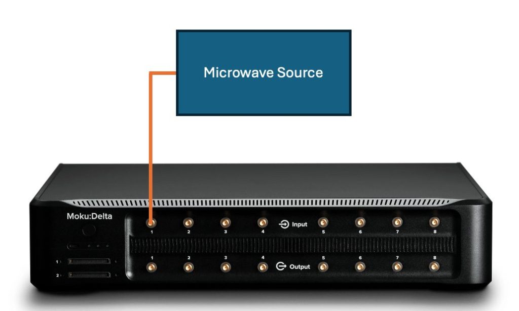
We use an external microwave generator with a range up to 12 GHz, attached to Input 1 on the Delta’s analog front end as seen in Figure 9. We want to characterize the quality of the microwave generator by examining the presence of spurs and harmonics at various output frequencies. We launch the Spectrum Analyzer instrument and view the results.
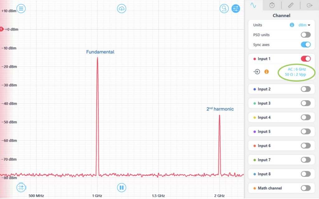
The first test is to generate single tones using the microwave and confirm that they alias at the expected frequency when undersampling mode. When using the Spectrum Analyzer in single-instrument mode, the option to enable 6 GHz can be found alongside other signal conditioning options on the right panel (see Figure 10). We begin by generating a continuous, 1 GHz tone with the microwave generator. As seen in Figure 9, since the fundamental frequency lies within the first Nyquist zone (up to 2.5 GHz for Moku:Delta), it appears at its “true” frequency of 1 GHz. The second harmonic (2f), also within the first Nyquist, appears at 2 GHz. Note that this harmonic is not introduced by Moku, rather it is a product of the microwave generator. The 3rd harmonic, at 3 GHz, would also alias at 2 GHz in this case. We can check this using Equation 3.
In this case, using the 6 GHz bandwidth mode on Moku:Delta is not advised, as the signal of interest falls within the first Nyquist zone, and the 2 GHz bandwidth cutoff is sufficient. Nonetheless, we can look at the spectrum of the signal and see that the 2nd and higher harmonics occur around ~30 dBc. Keeping in mind the frequency rolloff discussed in the previous section, we can determine that the power harmonic falls within the manufacturer’s specification.
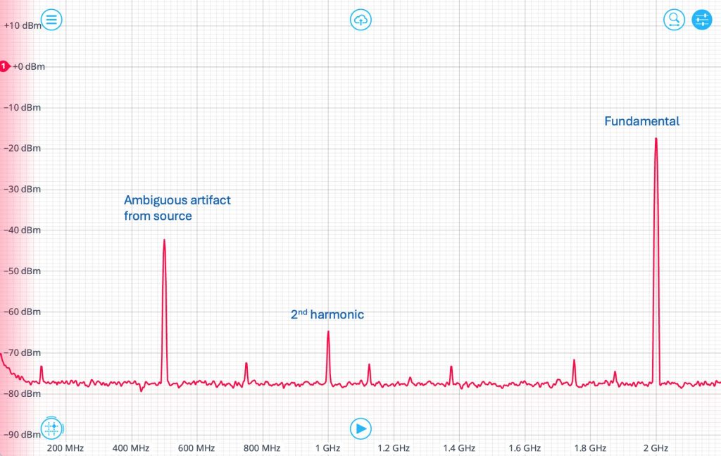
We now move to the second Nyquist zone and investigate the signal generator at 3 GHz. We expect the 3 GHz tone to alias at 2 GHz, which can be verified with Equation 3. The spectrum displayed in Figure 11 shows this behavior. The second harmonic, occurring at 6 GHz and aliasing to 1 GHz, is present at greatly reduced amplitude. This is due to the heavy attenuation by the Moku Delta frontend when approaching 6 GHz.
Examining the spectrum, we see a spur appear at 500 MHz, originating from the microwave source. However, when observed in the aliased domain alone, its true origin is not immediately obvious. Using Equation 3, we determine that a signal observed at 500 MHz and sampled at 5 GSa/s could correspond to a real signal at 4.5 GHz, 5.5 GHz, 9.5 GHz, or another frequency following the same pattern.
This illustrates an important limitation of undersampling: aliasing preserves spectral content but discards absolute frequency information. Without additional constraints, such as prior knowledge of the signal band or how spectral components move as the input frequency is varied, the true origin of aliased signals may be ambiguous. Care must therefore be taken when interpreting undersampled spectra.
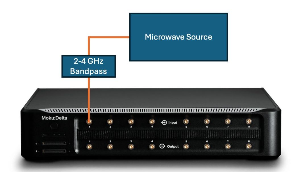
To investigate the origin of this spur further, we insert a 2-4 GHz bandpass filter in between the microwave source and Moku:Delta, as seen in Figure 12. This will help us to pinpoint the origin of the artifact, as it will be attenuated if it originates outside the 2-4 GHz band.
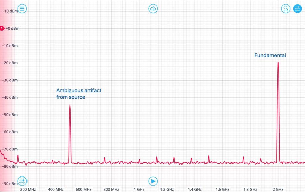
We look at again at the Spectrum Analyzer and see the result of the added filter, seen in Figure 13. The harmonic, occurring at 3 GHz, remains at its alias of 2 GHz with around 1 dB of attenuation. The 2nd harmonic, aliasing at 1 GHz, is no longer present in the spectrum, as it falls outside the bandpass filter. The artifact remains, with around 2-3 dB of attenuation. We can then deduce that the true frequency of this artifact is 4.5 GHz, as it lies just outside the passband of the filter and as such is not as attenuated a heavily as it would at 500 MHz or 5.5 GHz. This 4.5 GHz tone is likely a result of a fractional PLL divider inside the frequency source.
In this section, we’ve shown how to analyze spectra in higher Nyquist zones via undersampling. By combining the Spectrum Analyzer with a carefully chosen bandpass filter, we can isolate ambiguous frequency components and determine their frequency of origin. Provided that care is used when interpreting aliased spectra, undersampling can be an effective way to measure high frequency signals while preserving spectral content.
Conclusion
In this note, we discussed how to convert information from the analog to digital domain via sampling. We show how to utilize undersampling mode on Moku:Delta to increase the analog bandwidth of the Spectrum Analyzer and other instruments. While sampling below the Nyquist limit does preserve spectral information, it hides the absolute frequency origin. For this reason, as well as innate artifacts such as spectral mirroring, users should take care when analyzing such measured spectrums. For best practices, we recommend filtering around the bandwidth of interest and understanding the composition of the measured signals.