


In this application note we provide a tutorial using Moku:Lab’s Arbitrary Waveform Generator with MATLAB. Step-by-step instructions are detailed for deploying two simple waveforms from MATLAB directly to Moku:Lab. We use a second Moku:Lab running the Oscilloscope and Spectrum Analyzer instruments to confirm the output waveforms.
A Lissajous curve example is then shown together with a more complex, 2 channel waveform.
MATLAB files to accompany this note are available to download from Liquid Instruments.

Arbitrary Waveform Generator
Moku:Lab’s Arbitrary Waveform Generator (AWG) can generate custom waveforms with up to 65,536 points at sampling rates of up to 1 GSa/s. Waveforms can be loaded from a file, or input as a piece-wise mathematical function with up to 32 segments, enabling you to generate truly arbitrary waveforms. In this note we will generate the waveform and download it directly to Moku:Lab, entirely within MATLAB.Prerequisites and setup
This application note and tutorial assumes you have installed MATLAB and the associated Moku:Lab MATLAB toolbox : Moku:Lab supports the following MATLAB versions:- Windows: MATLAB R2013a and later
- Linux: MATLAB R2013a and later
- MacOS: MATLAB 2014a and later
- Download the Moku:Lab toolbox here: http://updates.liquidinstruments.com/static/moku-MATLAB-2.8.1.mltbx
- In MATLAB, open the downloaded .tblx file
- Select “Install”
- Confirm installation with help moku in the MATLAB terminal
- Download the Moku:Lab toolbox zip here: https://updates.liquidinstruments.com/static/moku-MATLAB-2.8.1.zip
- Extract the zip, typically to
../MATLAB/Add-Ons/Toolboxes - Open MATALB and, in the Home tool pane, click “set Path”
- Click “Add with Subfolders” and select the folder of the extracted ZIP
- Click “Save” to add the toolbox folder to the MATLAB path
Moku:Lab on MATLAB
In order for MATLAB to control Moku:Lab, the computer running MATLAB must be on the same sub-net/LAN as Moku:Lab. MATLAB needs the IP address of Moku:Lab; you can determine this in one of two ways :- A Bonjour/zeroconf service discovery utility
- On launch screen of Moku:Lab’s iPad app; push and hold the icon of the Moku:Lab to reveal its IP address
~/Library/ApplicationSupport/MathWorks/MATLAB Add-Ons/Toolboxes/moku-MaTLAB-2.8.1/examples
On Windows:
\Users\...\AppData\Roaming\MathWorks\MATLAB Add-Ons\Toolboxes\moku-MATLAB-2.8.1\examples
Downloads
The MATLAB scripts for each of these examples are available for download here: https://download.liquidinstruments.com/documentation/app-note/reference-files/20-0331_AppNote-MatLab-UsingAWG_ScriptsForMokuLabAWG.zipExample #1 : Square wave and sine wave with harmonics
For our first example we will deploy the Toolbox example:arbitrarywavegen_basic.m
Referring to this script, we see that the array square_wave is defined to be an array of length 100 consisting of values of +1 or -1.
The not_square_wave is defined to be an array of length 100 of values describing a sine wave with the addition of several odd-numbered harmonics.
After running the MATLAB script, the user enters an IP address and within the script, the line :
m = MokuArbitraryWaveGen(ip)
sets up and deploys an instance of an Arbitrary Waveform Generator instrument on Moku:Lab. Then one call for each channel to
m.write_lut
and
m.gen_waveformfunction
configures the waveform on the Moku:Lab hardware.
We can view and confirm these waveforms with the MATLAB plotting and graphing commands. Figure 1 shows the square wave in blue and the sine wave plus harmonics in red.
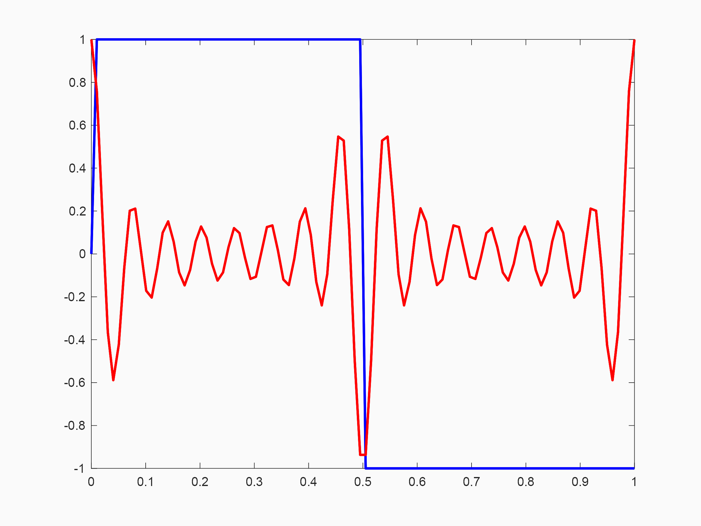
Figure 1: MATLAB plot of example waveforms
But, it is more useful to view these waveforms as generated on Moku:Lab. On our lab bench, the top, black Moku:Lab is connected to MATLAB and generating our two signals with the deployed AWG. The lower blue Moku:Lab is interfaced with an iPad, which is running the Oscilloscope instrument. This setup is shown in Figure 2.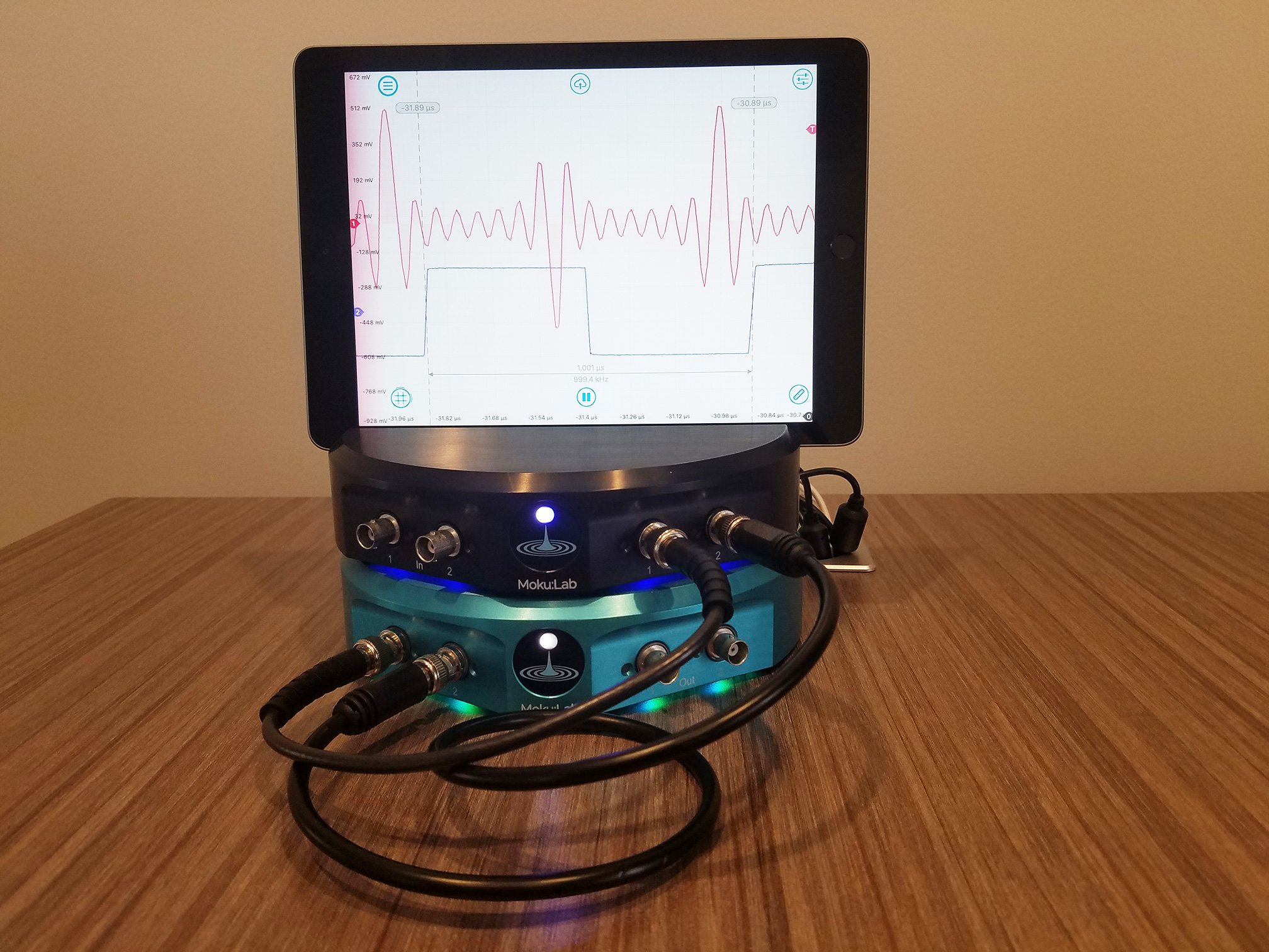
Figure 2: Moku:Lab setup
The AWG output channels are connected to the Oscilloscope inputs and we can observe the waveforms on the iPad. The cursors show the expected frequency of 1 MHz (actual measurement on screen of 999.4 kHz). Moku:Lab’s integration with Dropbox allows us to quickly share the screenshot, see Figure 3 (showing the actual AWG output), a square wave on channel 2 (blue), and a sine wave plus harmonics on channel 1 (red).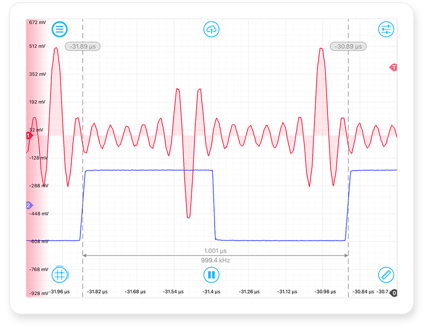
Figure 3: Moku:Lab Oscilloscope screenshot, shows the MokuLab AWG as generated from MATLAB
Due to Moku:Lab’s flexibility we can quickly switch the blue Moku:Lab from an Oscilloscope to a Spectrum Analyzer. The spectrum of the square wave shown in Figure 4 and as expected for a square wave, shows fundamental at 1 MHz and a series of odd harmonics extending to the limits of the plot at 100 MHz.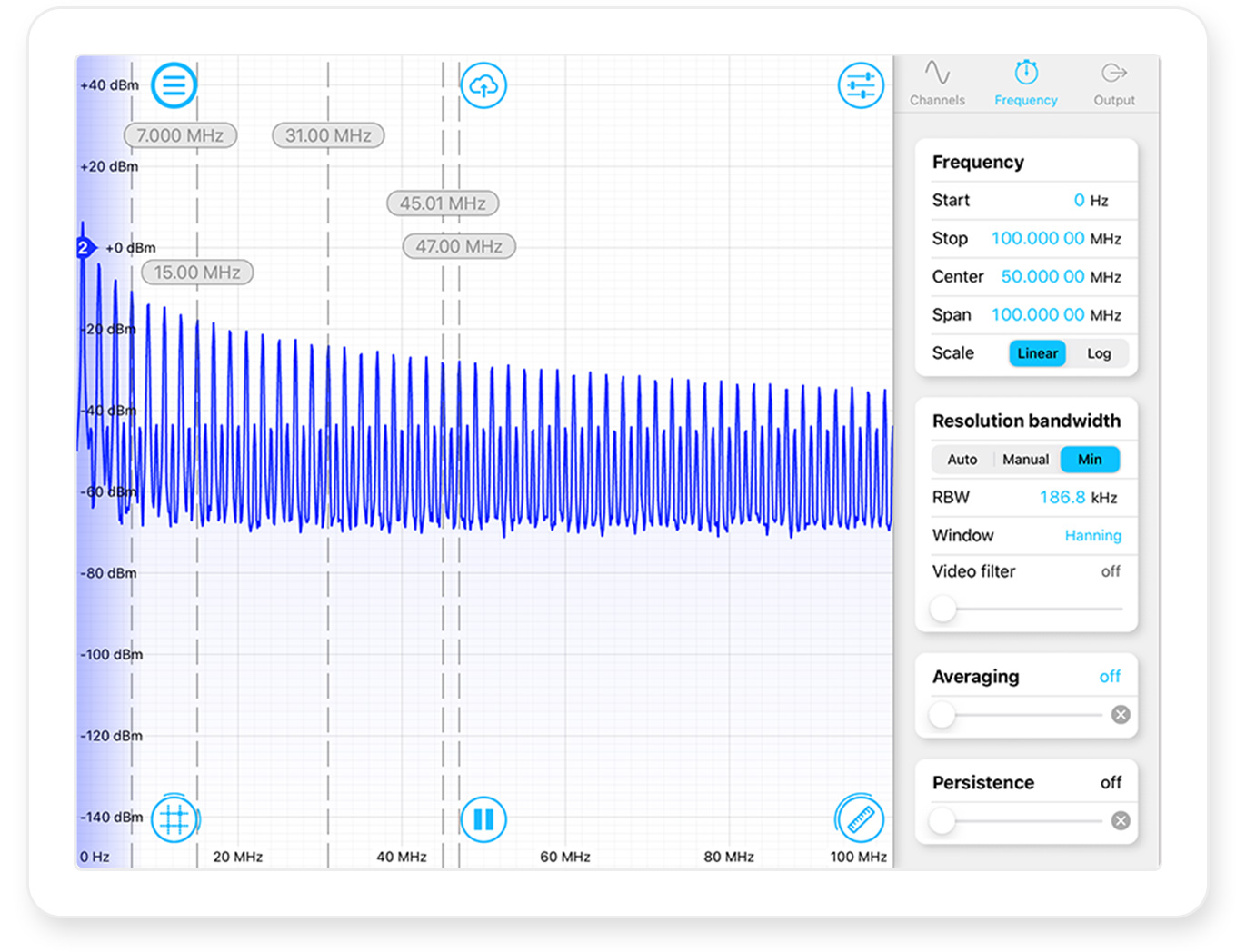
Figure 4: Square wave spectrum on Moku:Lab’s Spectrum Analyzer
Our MATLAB script for the not_square_wave essentially sums a sine wave with 7 odd harmonics. The spectrum of not_square_wave is shown in Figure 5 and this shows the 1 MHz fundamental and 7 harmonic peaks extending to 15 MHz. This is labelled on screen with a cursor from the iPad app.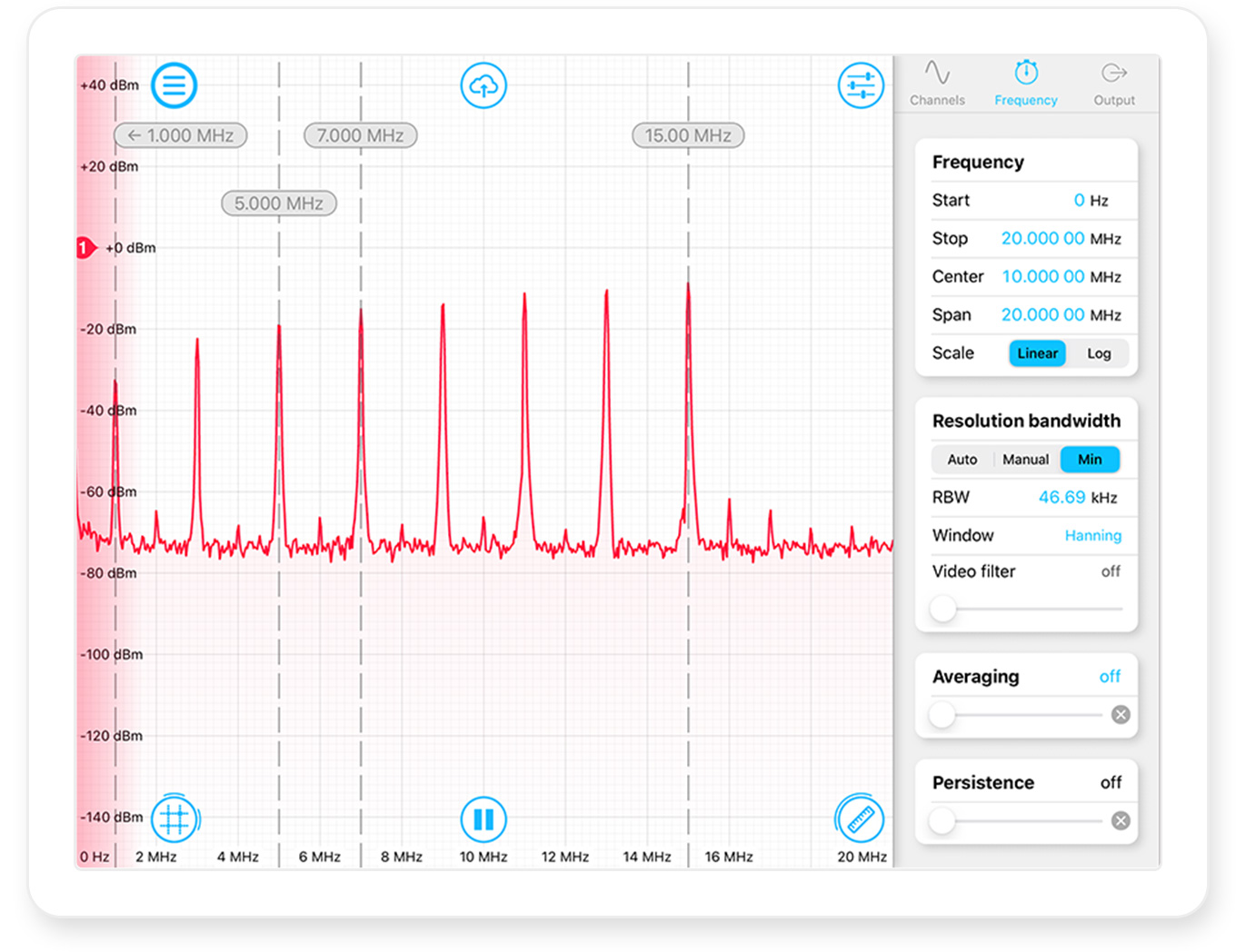
Figure 5: “not-square-wave” as seen on Moku:Lab Spectrum Analyzer
Example #2 : Lissajous figures
For a second example of Moku:Lab’s AWG, we will generate a classic Lissajous figure. Lissajous curves are defined in x and y as:x = Asin( at + d )
y = Bsin( bt )
This family of curves was investigated by Nathaniel Bowditch in 1815, and later in more detail by Jules Antoine Lissajous in 1857. By integrating some Moku:Lab API function calls into the MATLAB scripts from [3], we can define some waveforms and see the resulting Lissajous curves in MATLAB. This MATLAB script islissajous_moku.m
Once running, a GUI window opens in MATLAB and allows the user to configure the variables A, a, d, B, b and t. By clicking on “start”, MATLAB will plot the figures and then a few seconds later, download the waveforms to the connected Moku:Lab’s AWG. Figure 6 shows the MATLAB output and Figure 7 shows the output of Moku:Lab’s AWG as captured on the second Moku:Lab’s Oscilloscope operating in X-Y mode.
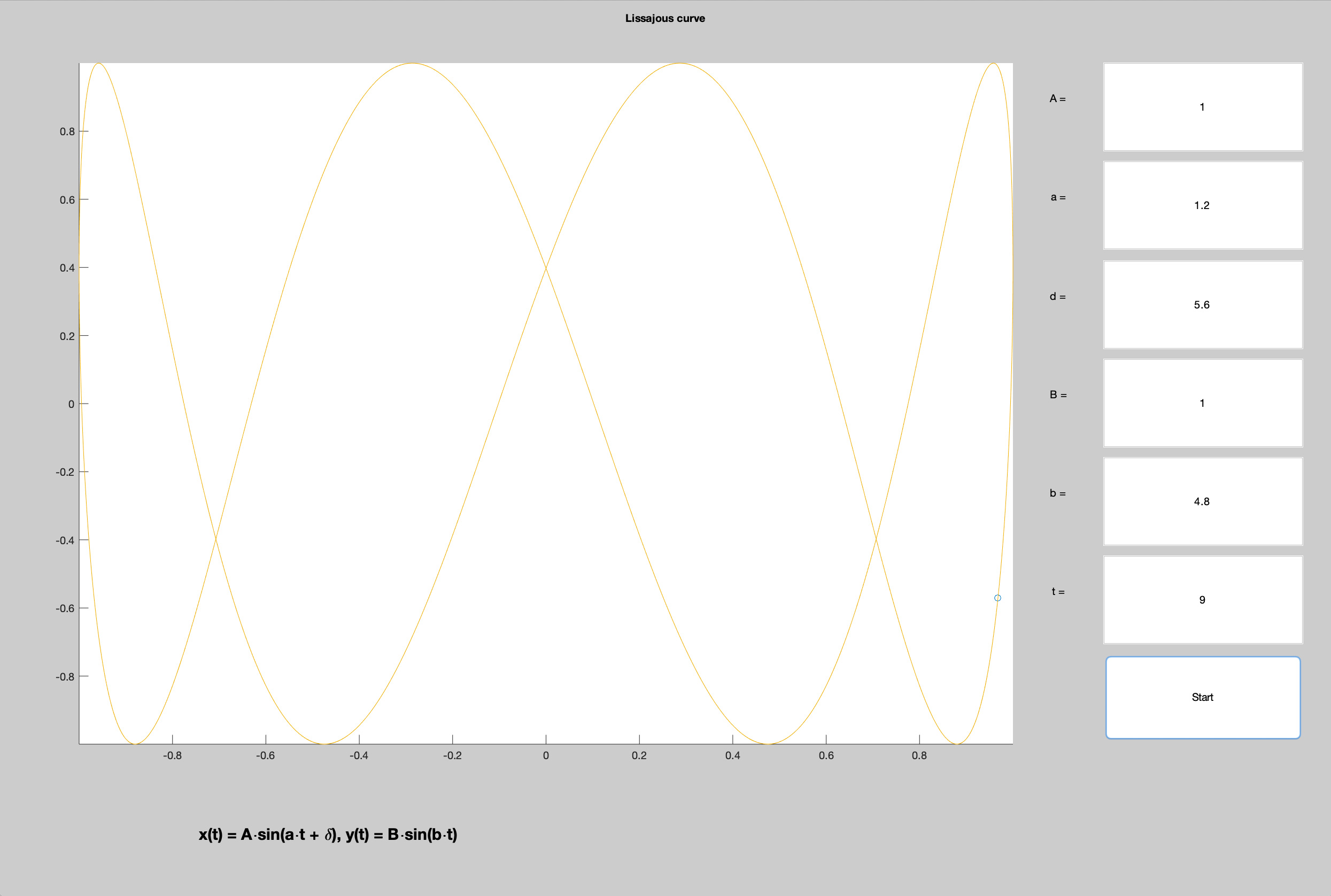
Figure 6: MATLAB Lissajous curve
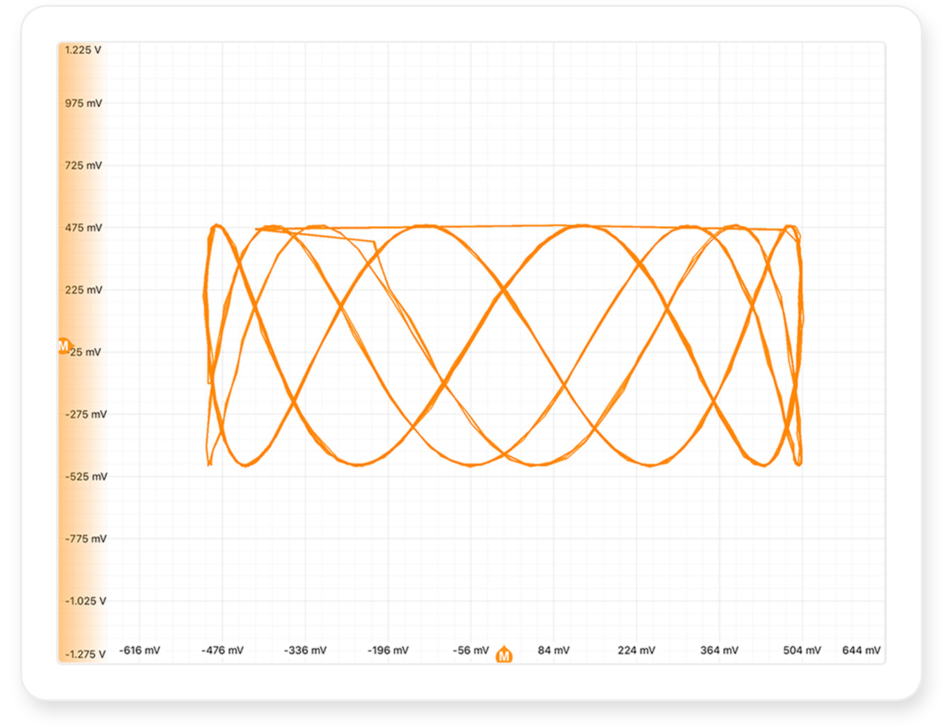
Figure 7: Moku:Lab’s AWG showing on Moku:Lab’s Oscilloscope