Introduction
Cross-correlation a useful technique in signal processing, essentially comparing the similarity of two signals. This technique eliminates the uncorrelated (random) noise between the signals, making it useful for accurate phase noise analysis by lowering the overall noise floor. It is also useful for matching signals in time, as it produces an amplitude maximum when the two signals overlap. This is a valuable feature in applications such as determining range or time-of-flight in radar measurements, or for comparing an incoming signal to a known template.
In this application note, we introduce the integral form of cross correlation and examine its physical meaning. We then discretize this expression and discuss its use in signal processing applications. Finally, we present the concept of cross-power spectral density, which is the equivalent of cross correlation in the frequency domain. We use the Moku Oscilloscope and Spectrum Analyzer to illustrate several examples of this concept.
Cross-correlation in the time domain
Integral form
Mathematically, cross-correlation is defined as the integral of the product of the two signals, which is then normalized. One signal is usually given a variable time delay \(\tau\), and the cross-correlation becomes a function of this time delay. Depending on whether the signals are of similar or opposite amplitudes, the correlation function can also take on positive and negative values. Start with two continuous, arbitrary functions \(y(t)\) and \(x(t)\), with the complex conjugate of \(x(t)\) represented by \(x^*(t)\). Averaging over some time \(T\), as a function of time delay \(\tau\):
\(R_{xy} = \frac{1}{T} \int^{T/2}_{T/2}{x^*(t)y(t+\tau)dt}\) (1)
Let us assume that \(x(t)\) and \(y(t)\) are strictly periodic over a period T, with arbitrary amplitudes and a phase difference between them.
\(x(t) = A \sin{(\omega t)}\) (2)
\(y(t) = B \sin{(\omega t + \phi)}\) (3)
Note that the complex conjugate of a real function such as \(x(t)\) is self-equivalent. We can then rewrite the definition of \(R_{xy}\) as:
\(R_{xy} = \frac{1}{T} \int^{T}_{0}{x^*(t)y(t+\tau)dt}\)
Walking through the calculation, we can then insert equations (2) and (3):
\(R_{xy} = \frac{AB}{T} \int^{T}_{0}{\sin{(\omega t)} \sin{(\omega t + \phi)} dt}\)
Rewriting in complex notation:
\(R_{xy} = \frac{AB}{T} \int^{T}_{0}{ \left( \frac{e^{i \omega t} – e^{-i \omega t}}{2i} \right) \left( \frac{e^{i \omega (t + \tau) + \phi} – e^{-i \omega (t + \tau) – \phi}}{2i} \right) dt}\)
\(R_{xy} = \frac{-AB}{4T} \int^{T}_{0}{e^{i \omega (2t + \tau) + \phi} – e^{-i \omega \tau – \phi} – e^{i \omega \tau + \phi} + e^{-i \omega (2t + \tau) – \phi} dt}\)
Since the terms containing t are periodic, time averaging over one full period will return zero, leaving only two terms:
\(R_{xy} = \frac{AB}{2} \left( \frac{e^{i(\omega \tau + \phi)} + e^{-i(\omega \tau + \phi)} }{2} \right) = \frac{AB}{2} \cos{(\omega \tau + \phi)}\)
The correlation function depends on both the time delay and phase difference of the signals. At zero-time delay (\(\tau = 0\)), the functions are perfectly correlated at \(\phi = 0\) and perfectly anti-correlated at \(\phi = 180\). At \(\phi = 90\), the correlation goes to zero as the functions are out of phase with each other (see Figure 1).
Discrete form
For digitally sampled data, such as that captured by an Oscilloscope, the formula above must be discretized. Assume that two captured spectra contain real values \(x[t]\) and \(y[t]\), where t is the index of the data point. The cross correlation takes the form:
\(R_{xy}[\tau] = \sum_t x[t] y[t+\tau]\)
where the parameter \(\tau\) represents the time shift between x and y in terms of number of points.
In practice, the data sets \(x[t]\) and \(y[t]\) are finite, and thus there is a limit on how much the functions can shift in time. At large offsets, the overlap between the data sets shrinks. For example, assume a set of \(x[t]\) and \(y[t]\) that are exactly 1000 points. While one can mathematically offset by \(\tau =999\) points, the overlap is then only one point in each set, and the result is a generally not a useful quantity.
The usual approach in this scenario is to acquire more data points than the desired window size. As a rule of thumb, the total length of the trace should be
\(N_{trace} = N_{window} + N_{lag, max} \)
This ensures the correlation function is fully populated without running into the edges.
For comparing amplitudes or phase shifts, it is common to subtract DC offsets from the traces, as well as normalize them by their RMS amplitudes. Therefore, the full form of the correlation function becomes:
\(C_{xy}[\tau] = \frac{\sum_t{(x[t] – \bar{x})(y[t+\tau]-\bar{y}_m) }}{\sqrt{\sum_t{(x[t]-\bar{x})^2}} \sqrt{\sum_t{(y[t+\tau]-\bar{y}_m)^2}} }\)
Where \(\bar{x}\) and \(\bar{y}_m\) are the means of \(x[t]\) and \(y[t+\tau]\) over the overlapping window. This gives a normalized correlation that is always between -1 and +1, independent of amplitude.
Measuring cross-correlation with the Moku Oscilloscope
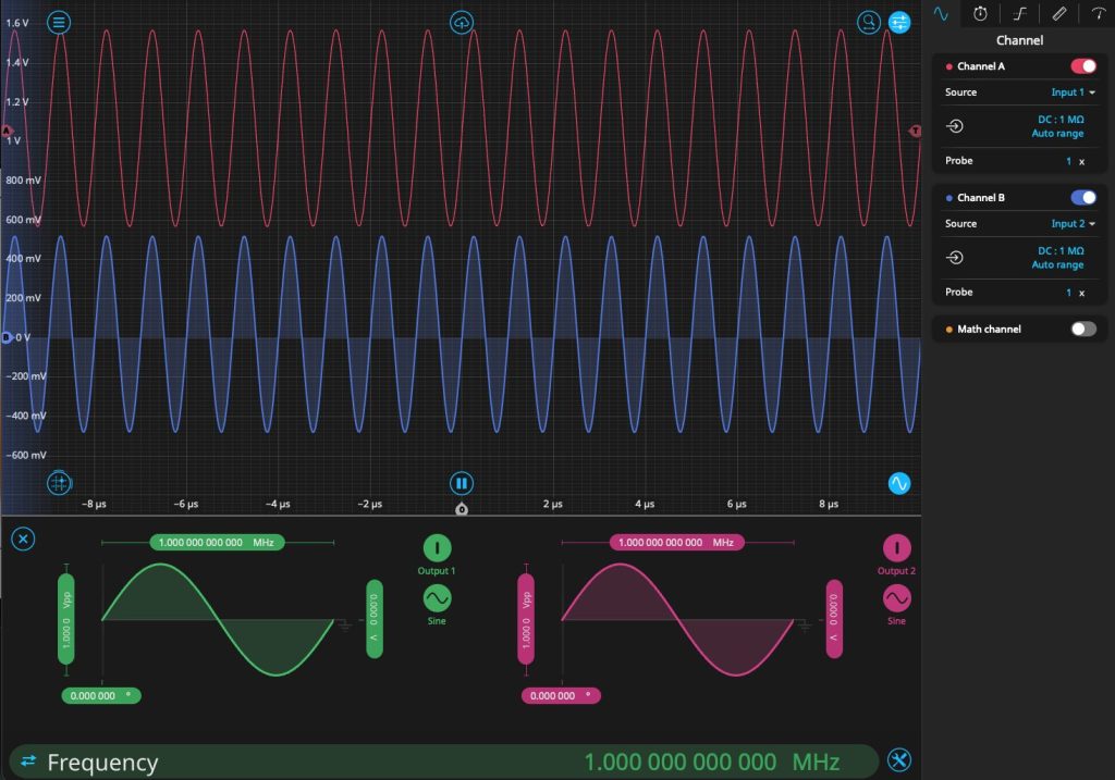
We first demonstrate cross-correlation on Moku by taking traces from the Oscilloscope and manually calculating its cross-correlation value with a Python script. Using a Moku:Go, we connect OutputA to InputA and OutputB to InputB with BNC cables of matching length. We then launch the Moku software in Oscilloscope mode and use the embedded Waveform Generator to output two matching sine waves, as seen in Figure 1 below.
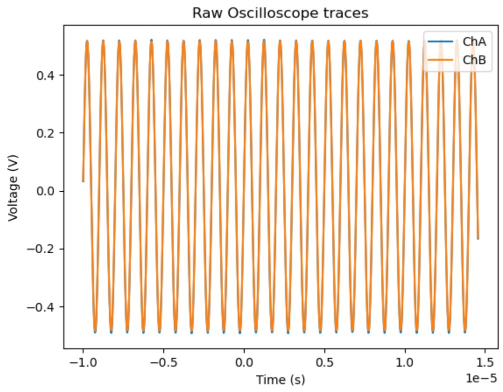
We now move to Python. We automate this measurement by configuring the Oscilloscope settings and capturing the traces. For information on the Moku Python API, please see the documentation. Each trace consists of 1024 points, controlled by the set_timebase command. To verify that the script is collecting the data as expected, we plot the results in Figure 2.
Next, we calculate the cross-correlation plot by creating a function that slices each vector by N points and then multiplies the remaining data together. Normalizing appropriately, as per the equation for \(C_{xy}\) above, we obtain the plot seen in Figure 3.
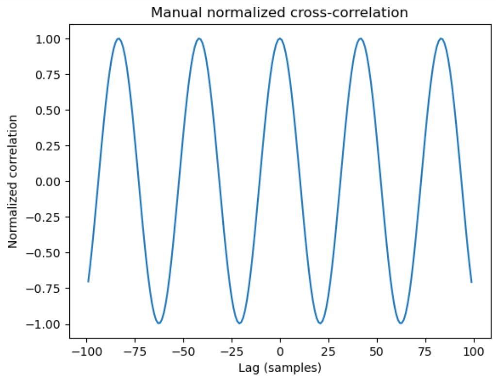
The cross-correlation plot oscillates between +1 (perfect correlation) to -1 (perfect anticorrelation) as a function of lag. At zero lag, the correlation is +1 because the original signals are phase coherent; applying a phase shift will shift the values of the cross-correlation plot to the left or right. It will, however, remain periodic as long as the input signals are periodic. The period of this oscillation is approximately 42 samples, which means that shifting the signal on Channel B by 42 samples will result in the same value of cross-correlation due to the periodic nature of signals. The value of 42 samples depends on the sampling rate of the Oscilloscope and the size of the collected array.
Calculating cross-spectrum from time-series data
Having calculated the cross-correlation of the time series data, we can use the same Oscilloscope configuration to calculate the correlation in the frequency domain. In the frequency domain this quantity is usually called the cross-spectrum, or occasionally the cross-power spectral density, and gives information as to how the correlation is distributed over frequency space. First, we transform the discrete time series data sets \(x[t]\) and \(y[t]\) into the frequency domain via a Fourier transform. We write these quantities as \(X[f]\) and \(Y[f]\), respectively. To measure the phase relation between the two signals, we take the complex conjugate of \(Y[f]\), then normalize by the number of points N. This gives us a quantity that has units of voltage square, allowing us to compare it to the power spectrum of the original signal, while preserving phase information. The equation for the cross-spectrum is given by:
\(S_{AB}(f) = \frac{X[f] \times Y^*[f]}{N^2}\)
Note that the above quantity is, in general, complex. In order to render it in the Moku Spectrum Analyzer alongside other spectral data, we take the magnitude and convert it to a logarithmic scale, assuming a 50 Ohm impedance and using the following formula:
\(P_{dBm} = 10 \log_{10} \left( 0.001 \times \frac{|S_{AB}|}{50 \Omega}\right)\)
This has the unfortunate effect of removing the phase information from the displayed quantity; however, it remains in the full complex-valued expression \(S_{AB}(f)\). As seen in the next section, this remains a useful tool for removing noise and quantifying time-sensitive signals.
Cross correlation using the Moku Spectrum Analyzer
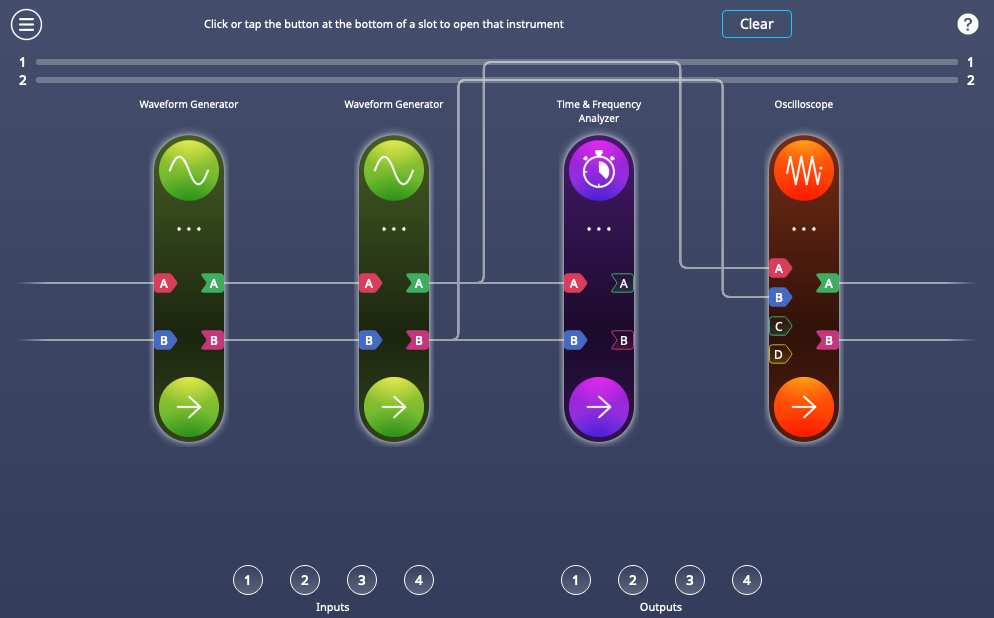
We will now work through a simple demo to test the cross-correlation function on Moku. In Multi-Instrument Mode, we place the Waveform Generator in Slot 2, the Spectrum Analyzer in Slot 3, and the Oscilloscope in Slot 4, as seen in Figure 4. This allows us to monitor the output from the Waveform Generator in both the frequency and time domain simultaneously.
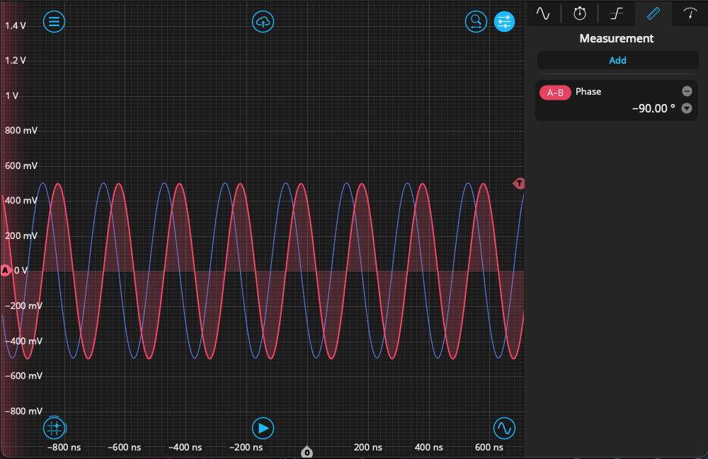
Opening the Waveform Generator, we create two sine waves with a 5 MHz frequency and a relative phase of 90°. We synchronize the phase and move to the Oscilloscope to view the signals in the time domain. As can be seen in Figure 5, the signals are matched in amplitude with a phase offset between them.
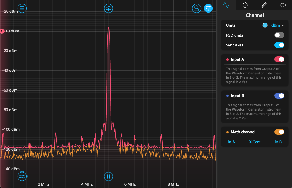
We now move to the Spectrum Analyzer and view the signals in the frequency domain over a span of 10 MHz, as seen in Figure 6. As they originate from the same source, both signals look similar – featuring the same spurs and other characteristics of a digitally generated signal. Enabling the math channel and cross-correlation feature, we can see that the noise floor is generally lowered, but the main signal and spurs are preserved. This is consistent with our understanding of cross-correlation, as uncorrelated features are suppressed, while common components of each signal are preserved.
As we determined in the previous section, this feature takes the magnitude of the calculated cross spectrum and discards the phase information, meaning that the 90° phase difference between the two signals is not reflected. To show how cross-correlation can determine the temporal sameness of two signals, we return to the Waveform Generator and generate two chirp pulses, ranging from 5 MHz to 50 MHz. The configuration is seen in Figure 7. Both signals begin at 5 MHz and sweep in sync over a period of 5 ms.
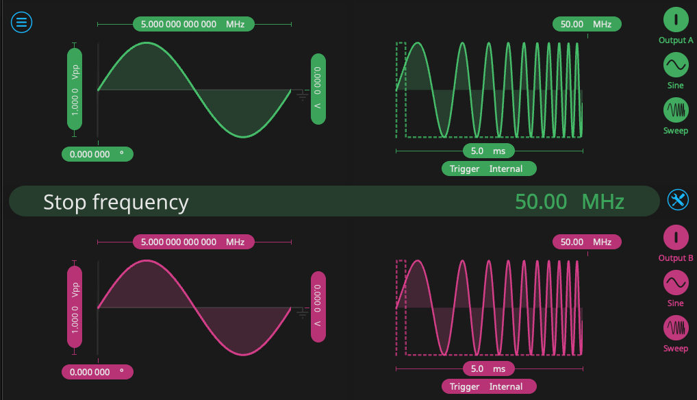
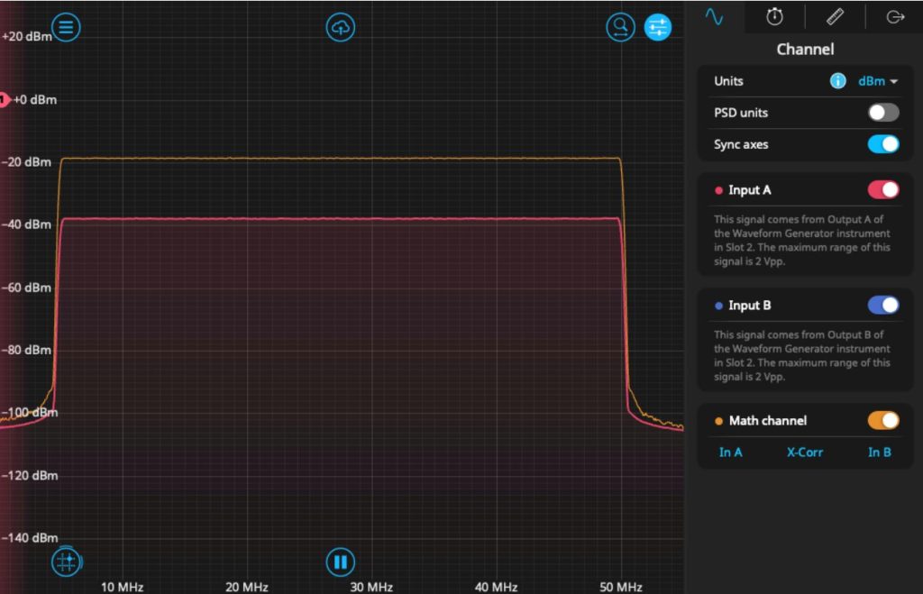
Looking at the output of the Moku Spectrum Analyzer, we see that both signals are visible as a plateau in frequency space, with sharp dropoff below 5 MHz and above 50 MHz. Both sweeps appear close to identical, overlapping neatly in the plot, while the calculated cross-correlation indicates that the signals overlap in time.
We show the usefulness of the cross-correlation by reversing the direction of one of the chirps, sweeping from 50 MHz to 5 MHz over the same time period, while keeping the channels in sync. In frequency space, this looks identical as the Fourier transform does not take into account the direction of the sweep. This can be seen in Figure 9. Input A and B do not change from the previous case and overlap on the Spectrum Analyzer screen. The cross-correlation, however, reflects this change because it is dependent on the instantaneous frequencies of each signal. While previously a plateau, the cross correlation plot has been reduced by around 50 dB, only peaking around 25 MHz. This is the point where the sweeps meet, overlapping in frequency for a brief period of time before continuing in opposite directions.
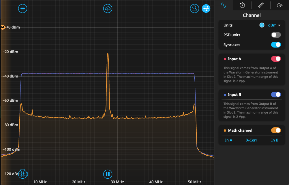
Although the Spectrum Analyzer operates in the frequency domain, the addition of cross correlation effectively restores sensitivity to time-dependent behavior. Signals that are indistinguishable in magnitude spectrum alone can be clearly differentiated once their temporal overlap is considered.
Conclusion
Cross-correlation provides a powerful way to compare the similarity of two signals, reject uncorrelated noise, and extract timing or phase relationships with high precision.
In this application note, we began with the integral definition of cross-correlation and explored its physical interpretation. We then examined the cross-power spectral density, the frequency-domain counterpart of crosscorrelation. Finally, we demonstrated how these concepts appear in real measurements using the Moku Oscilloscope and Spectrum Analyzer. Together, these tools illustrate how cross-correlation techniques can enhance measurement accuracy across a wide range of applications.