Part 2: Feedback control

2.1 Introduction

Part two of our series on frequency-domain control demonstrates how one can construct feedback control loops using the block-diagram approach discussed previously. Please see Part 1 for an introduction to the mathematical representation of our control loops. We will analyze these loops and discover how they can track a changing set point or mitigate disturbances. As an example, we will look at disturbances arising from the loop sensor itself.

Part 1 establishes the definition of a transfer function and provides the components from which one can construct control loop block diagrams to model elaborate systems. In part 2 we demonstrate how feedback control systems can be used to suppress disturbances or track a process set point. The complications associated with noisy sensors are also discussed. Unlike open-loop systems, devices under feedback control have the potential to become unstable and there is tension between performance and robustness. Ultimately, delays in signal propagation can impose the most stringent limit. These issues are treated in part 3. In the frequency domain, most parameters of a feedback system can be linked to its open-loop transfer function. In part 4 we explain how to measure this important quantity and provide a list of functions often used in shaping it. Part 5 describes one method of avoiding actuator saturation and, in doing so, introduces ideas useful to the treatment of multiple actuators. Our series concludes in part 6 with the study of the PID controller. This common control architecture is generally considered from a time-domain point-of-view; we illustrate the complementary frequency-domain representation.

2.2 Open loop

Let us begin our foray into the world of control systems proper by considering the frequency control system of Figure 2.1. Such a diagram could represent the tuning input of a voltage-controlled oscillator (VCO), laser, or motor (in which case we’d think of frequency as rotation rate or speed). The system to be controlled is often called the plant.

Figure 2.1: An open-loop frequency control system. H(s), with dimensions of Hz/V, describes the transfer function of the system’s tuning input. In response to a set-point input of X_sp, the output frequency is , i.e. .

Ideally, one could simply fix the input voltage based on the desired output frequency, varying it as necessary. Unfortunately, real-world disturbances render this approach unfeasible. We divide disturbances into input and output categories as shown in (see Figure 2.2).

Figure 2.2: Input and output disturbances, di and do respectively, perturb the system. This necessitates action on our part to maintain the desired output. Note that in the interest of brevity and readability, we henceforth omit dimensions and independent variables.

Under closed-loop control, the effect of input and output disturbances can be quite different and the distinction between them relatively subtle. Considering the dimensions of the disturbance and whether it should be filtered by the transfer function in question usually removes any uncertainty.

2.3 Feedforward

A simple approach to combatting a disturbance would be to:

• Characterize the effect disturbances of this type have on the system
• Accurately measure the disturbance
• Adjust the set point to cancel the effect of the disturbance

Suppose that the system of Figure 2.1 is perturbed by an output disturbance, e.g. temperature (Figure 2.3, top). Said disturbance modifies the output frequency via the system’s response to temperature R [Hz/K]. The resulting output is

In hopes of mitigating the perturbation, we measure the ambient temperature using a sensor with transfer function S [V/K] and implement a model of our system M [V/V] (Figure 2.3, bottom). Subtracting the output of the model from the system input we find that

Thus, if M = R/SH, we can theoretically rid our system of the influence of temperature. This is the essence of feedforward control.

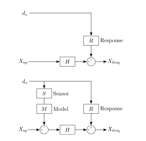
Figure 2.3: Feedforward is an open-loop technique which relies on canceling the effects of a disturbance (temperature, for example) by measuring it and having prior knowledge of how it impacts the system.
Feedforward is a powerful, generally stable, open-loop technique which allows disturbances to be corrected before they are able to influence system output. However, feedforward demands precise knowledge of one’s system, in terms of both the plant and the disturbance. Any unmodeled disturbances or temporal variability in the system results in markedly reduced performance. Hence, the technique is often confined to well-characterized, predominantly industrial, processes where the disturbances are predictable factors such as changes in set point or the opening of valves rather than quasi-random environmental influences. Operation in tandem with feedback can circumvent some of these drawbacks, but that is outside the scope of this work.

2.4 Feedback

An alternative approach to the treatment of disturbances is to

• Measure system output
• Compare the output to the desired value
• Adjust the set point until the desired output is achieved

Figure 2.4: Combating an output disturbance with feedback.

Such an approach is depicted in the upper diagram of Figure 2.4. Moving clockwise from the output, X_freq, the output is measured by a sensor with transfer function S, the difference between the sensor output and the requested set point is then computed at the summing node. We call this difference the error signal, ε. The error signal is then taken as the input to the system. If the output matches the set point, the error signal will be zero and the output of the system will not be modified. If the output is larger than the desired set point the error signal will be negative and act to reduce the output. Similarly, if the output is too small the control loop acts to increase the output.

This negative feedback loop is not, in general, stable (see §3.2). To ensure stability and to enable modification of frequency-dependent closed-loop gain, we introduce a controller, with transfer function C (Figure 2.4, bottom). The output of the controller, c, is known as the control signal and it is this quantity which acts on our system. The steady-state output is given by

(2.1)

Rearranging terms, we find (2.1) where we have introduced the open-loop transfer function, or OLTF, G, obtained by breaking the loop at any point and taking the product of all transfer functions met on moving around the (now open) loop. In this instance G = CHS.
Note that the numerator of the transfer functions encompasses the blocks encountered on moving from the input to the output and the denominator is 1+G. This realization provides a means of constructing transfer functions by inspection.
Study of (2.1) reveals the two key features of feedback control loops.

Reference tracking: The transfer function between the set point and the sensor output is

for large G.

so that the measured system output tracks the desired output (set point) where G is “large”. We define the concept of unity gain frequency, or ωUGF, to be the frequency at which |G| = 1. Roughly speaking, in practice, tracking is good for ω < ωUGF.

Disturbance rejection: The transfer function from disturbance to output is

for large G.

Thus disturbances are suppressed by a factor of approximately 1/G.

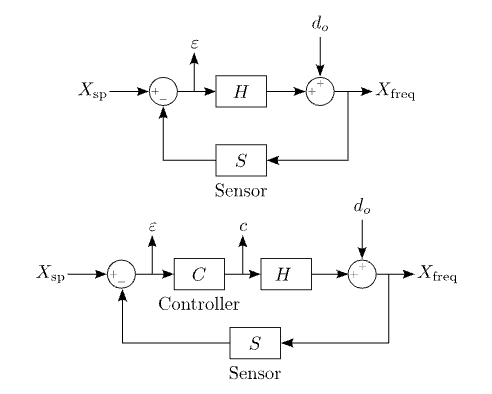
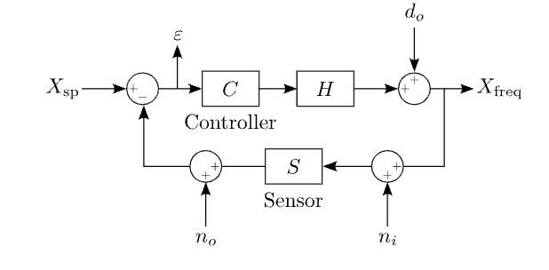
Figure 2.5: Input, n_i, and output, n_o, sensor noise directly limits loop performance.

2.5 Sensor noise

We can repeat the above procedure to compute the effect of disturbances introduced at any point in the loop. One type of disturbance, however, merits special mention – sensor noise.

We can consider two types of sensor noise, as seen in Figure 2.5. The first is input noise, n_i, which experiences the transfer function of the sensor, such as cavity length noise in a laser frequency stabilization setup. The second is output noise, n_o, which does not (e.g. most electronics noise).

It stands to reason that if our ideal picture of a system is corrupted due to a noisy sensor, our ability to achieve our control objectives will be compromised. This supposition is borne out by the following transfer functions relating sensor noise to system output,

We see that there is a clear path from sensor noise to system output. For input sensor noise in particular, the coupling is 1:1 where open-loop gain is high. To cement this idea, consider the example of a temperature sensor that reads consistently high by one degree. With our set point at 21 degrees, the loop will act to make the sensor output 21 degrees. However, due to the sensor error, the room will actually be at a temperature of only 20 degrees. The one-degree sensor error has been transmitted directly to our controlled variable.

The best we can hope for using a feedback control loop is to suppress disturbances down to the sensor noise. It may seem obvious, but is worth explicitly stating, that open-loop systems do not suffer from sensor noise.

A second issue with sensor noise comes when attempting to evaluate performance. Since the loop does not distinguish between sensor noise and true sensed output, the loop imprints sensor noise on the system output to reduce the ‘as-measured’ fluctuations. For example, if our sensor suffers from a 10 Hz noise oscillation, the loop will cause the system output to oscillate at 10 Hz in such a way that the sensor output is flat. In effect, the loop suppresses the sensor noise in the sensor output. If we then use the in-loop sensor to evaluate performance, we will see that it is flat and assume the output is stable, whereas in reality it is not. For this reason, an independent out-of-loop sensor is often employed, which can detect these types of issues.

2.6 Summary

Above we have introduced some of the fundamental features of feedback control loops. In contrast to feedforward loops, feedback loops are robust to parameter variations and do not require knowledge of the origins and coupling of each disturbance. Moreover, we also do not need an ideal model of our plant to achieve good performance. Stability, however, is not guaranteed and this topic will be the subject of our next installment – please see [Part 3].