Lock-in Amplifier configuration guide

Lock-in amplifiers (LIAs) are widely used instruments that can extract a signal of a known frequency that is overwhelmed by noise. A LIA mixes the signal with a local oscillator (LO) and uses a lowpass filter to reject the noise at unwanted frequencies. This allows the LIA to detect not only the amplitude but also the phase of the signal in relation to the LO. In this document, we will walk you through how to configure Moku:Lab’s LIA to detect the amplitude and phase of a weak 50 kHz signal with an external reference.

Signal and Reference Source

In this example, we used a second Moku:Lab’s waveform generator to simulate the signal and external reference for the LIA. A 50 kHz 1 mVpp sine wave was used as the signal, and a 50 kHz 500 mVpp square wave was used as the reference. (Figure 1) The signal and reference were generated based on the same clock (phase-locked), with an arbitrary phase relation to each other. This is a typical situation for a real experiment setup. Different electronic components have different instrument response functions and delays, which result phase difference between the signal and reference. The signal was connected to Moku:Lab’s LIA’s input 1, and the reference was connected to Moku:Lab’s LIA’s input 2.

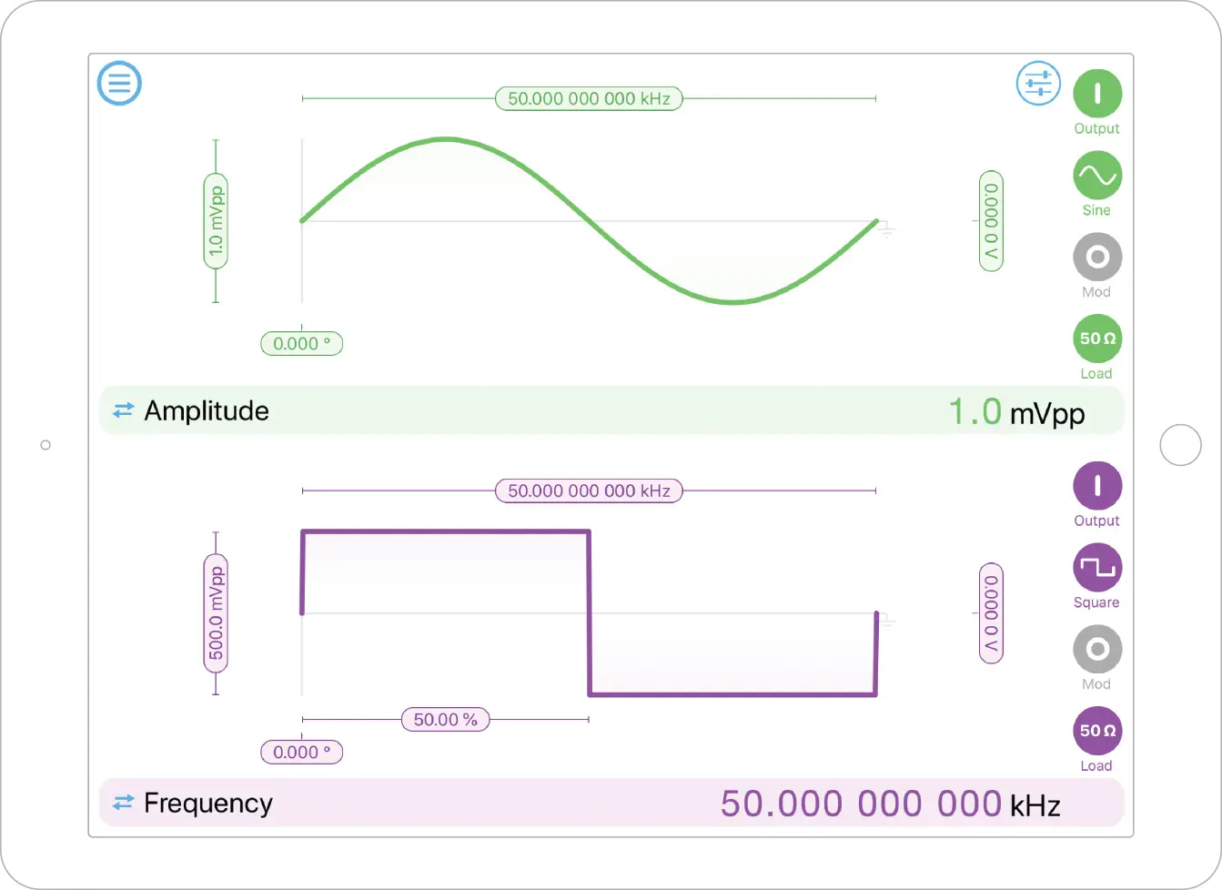
Figure 1: Waveform generator settings for signal and reference generation

Configure LIA’s Local Oscillator (LO)

LIAs extract the amplitude and phase of the signal with respect to the LO. It’s crucial to ensure the LIA uses the correct LO for the demodulation process. In this example, we used Moku:Lab’s LIA’s built-in phase-locked loop (PLL) to track the phase and frequency of an external reference source and generated two phase-locked orthogonal sinusoidal LOs for the dual-phase demodulation. First, we configured the LIA’s LO to the external (PLL) mode and output to filtered signal for simultaneous X/Y or R/θ detection. (Figure 2)

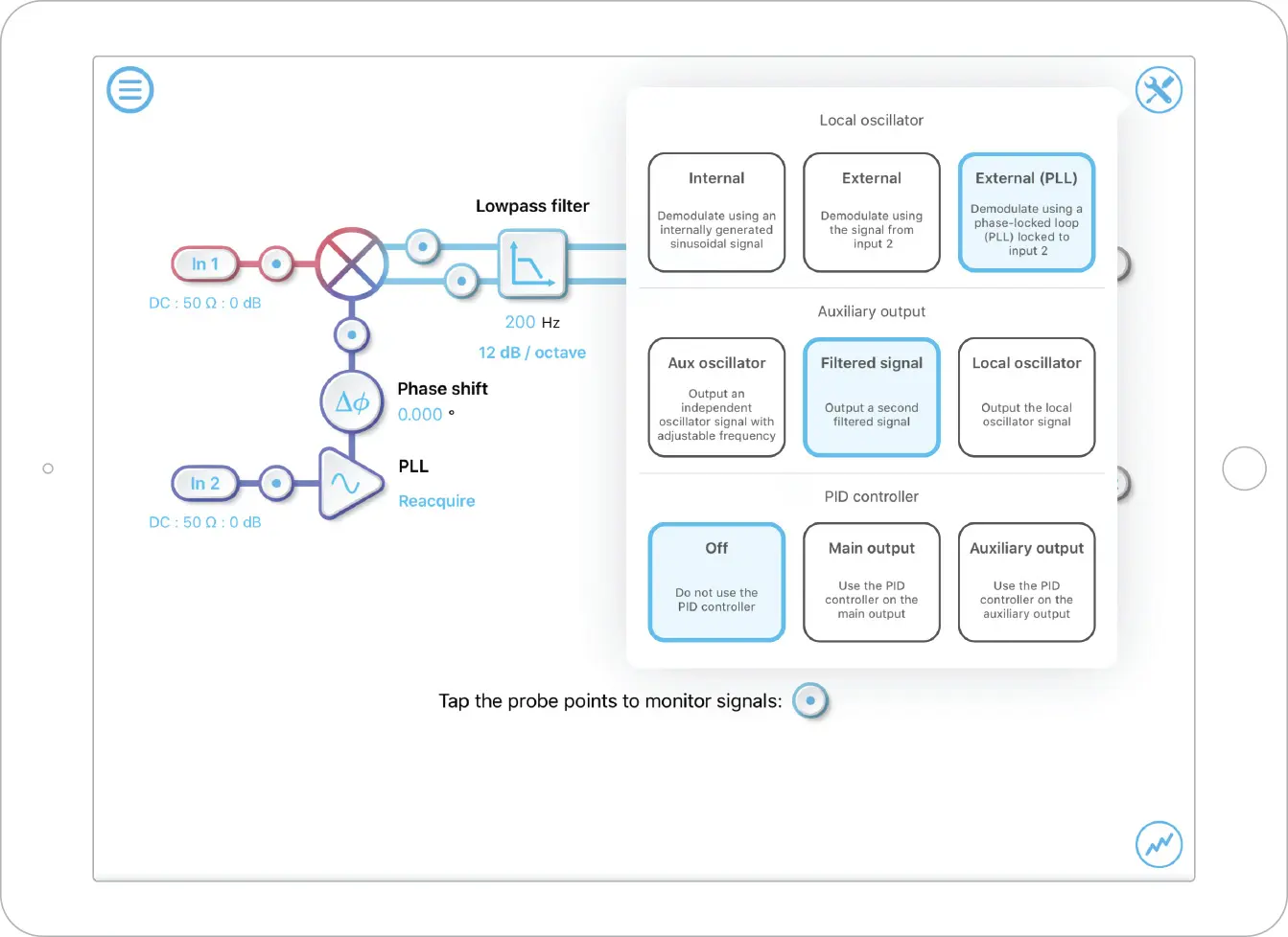
Figure 2: LO and auxiliary output settings for Moku:Lab’s LIA

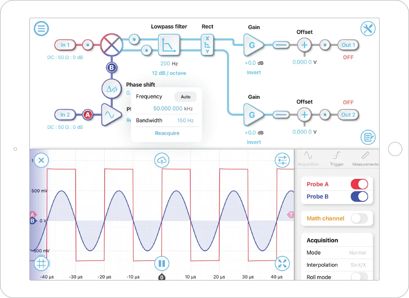
Figure 3: The undistorted sinusoidal LO (blue trace) phase was phase-locked to the reference input (red trace)

Configure the Lowpass Filter

The bandwidth of the lowpass filter significantly affects the SNR of the measurement. In general, a narrower bandwidth provides better noise rejection. However, narrow bandwidth also rejects any high-frequency component of the signal itself, which reduces the time resolution of the measurement. In this measurement, we expect a relatively steady sinusoidal output from the waveform generator. We set our filter bandwidth to 200 Hz, with a 12 dB/Octave slope.

Configure LIA’s Output Gain

Once the LO was set, we enabled the probe points for the X/Y output. Then, we increased the output gain to about +60 dB to bring the signal to a few hundred mV range. (Figure 4) This was similar to the sensitivity settings on some other lock-in amplifier, which allowed Moku:Lab’s LIA output DAC to fully unitized its resolution and range. To avoid saturation, the sum of the X² and Y² should be kept below 1 V.

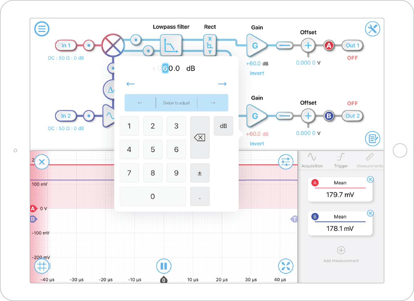
Figure 4: Moku:Lab’s LIA output gain settings

Adjust PLL’s Phase Shift

As we briefly mentioned before, the reference signal and the actual signal might have a significant phase difference. If the absolute phase shift is measured, it’s important to align the phase of the LO and signal. To align the phase, the phase shift of the PLL was adjusted to make the Y component as close to zero as possible. (Figure 5)

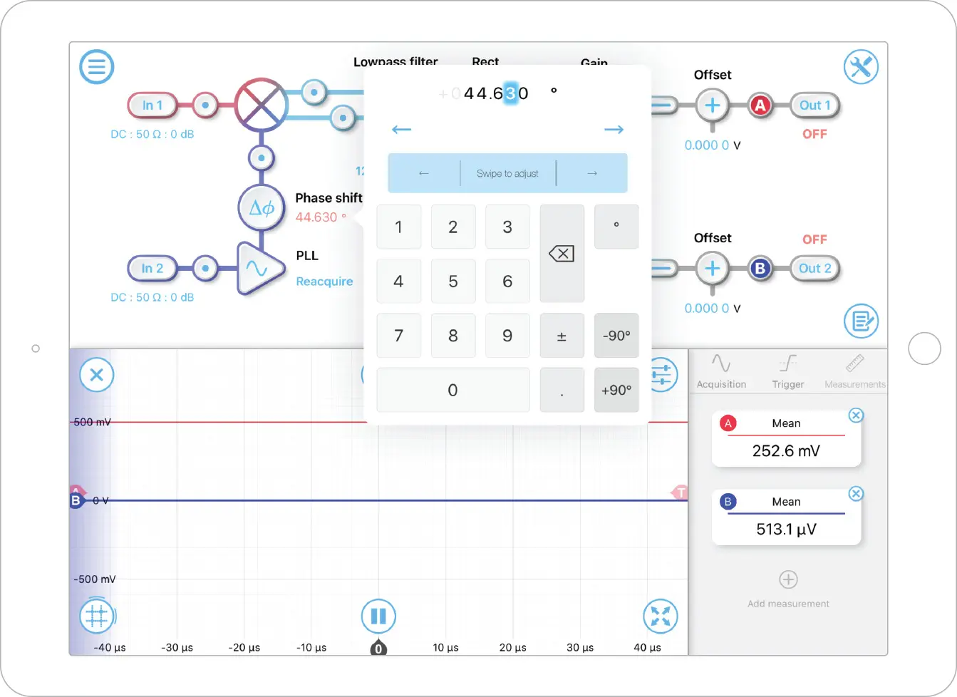
Figure 5: The phase shift of PLL was adjusted to 44.630 degrees to null the Y signal

Adjust Polar-to-rect Conversion Range

Last, we changed the output from X/Y mode to R/θ mode and adjusted the rect-to-polar conversion range. Optimal performance is achieved by choosing the smallest range which can accommodate your signal without saturating. Based on the X/Y mode, we estimated the output amplitude to be around 250 mV. We circled around the thee conversion range settings, and the 7.5 mVpp provided the best result. (Figure 6)

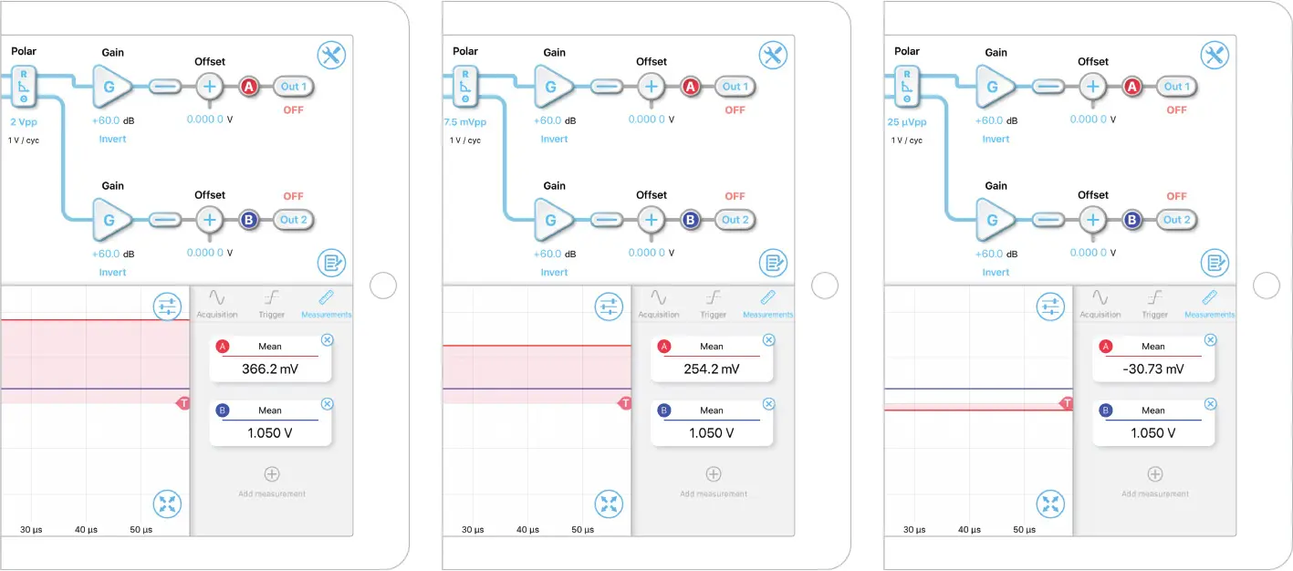
Figure 6: Optimizing the polar-to-rect conversion range based on the R output

Have questions or comments?

Contact us