

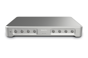

Through this demonstration, we showcase the effectiveness of Moku:Pro in rapid signal detection applications. You can also use a tool like an Autoencoder with the Moku Neural Network.
Introduction to the matched filter
Improving the signal-to-noise ratio (SNR) in communication and radar systems is a critical requirement for enhancing detection accuracy. The matched filter is a widely employed technique to improve SNR performance when the shape of the waveform of interest is known. This contrasts with conventional filters with passbands and/or stopbands defined in the frequency domain, or the boxcar averager, which aims to eliminate time-domain elements. This application note provides a detailed exposition on the theory behind the matched filter. Additionally, we demonstrate two applications of the matched filter on Moku:Pro.Background

Derivation of the matched filter
Derivation based on continuous signals

 is typically assumed to be additive white noise, with its power spectral density (PSD)
  being independent of frequency. Following this fundamental principle, the expected power of is constant in time, with an expected power of is constant in time, with an expected power of
  resulting from the multiplication of the PSD of the noise signal
  and the PSD of the receiving filter
  The power of the received signal
  at time
  varies with the sampling time due to the non-time-invariant nature of the PSD of the transmitted signal. The PSD is given by
  . such that:
 Therefore, the SNR at
  denoted
  can be expressed as:
 To solve Equation 2.1.3 and find the condition for optimized SNR, we apply the Cauchy-Schwarz inequality. The condition for maximized SNR performance for a known transmitted signal is shown in Equation 2.1.4.
 And the derived optimal filter, i.e., matched filter is given in Equation 2.1.5.
 Where
Where  and
and  is the length of the signal. The choice of
  leads to a filter with the shortest delay while still being casual. Additionally, the constant multiplier
  scales the noise and single equally and can therefore be omitted from the analysis.
Extension to a digital system
The expression in Equation 2.1.5 is the optimal filter in continuous time. To give a quantitative comparison, we will now analyze the SNR performance of the discrete time digital system. In Equation 2.2.1, the length of the matched filter is and the expected noise power is
 ![E(|n_{o}[tau ]|^2)](https://s0.wp.com/latex.php?latex=E%28%7Cn_%7Bo%7D%5B%5Ctau+%5D%7C%5E2%29&bg=ffffff&fg=000&s=0&c=20201002) . The formula considers the the digitized channel noise
. The formula considers the the digitized channel noise ![n[tau ]](https://s0.wp.com/latex.php?latex=n%5B%5Ctau+%5D&bg=ffffff&fg=000&s=0&c=20201002) , matched filtered noise
, matched filtered noise ![n_{o}[tau ]](https://s0.wp.com/latex.php?latex=n_%7Bo%7D%5B%5Ctau+%5D&bg=ffffff&fg=000&s=0&c=20201002) , and matched filter’s impulse response
, and matched filter’s impulse response ![h[tau ]:](https://s0.wp.com/latex.php?latex=h%5B%5Ctau+%5D%3A&bg=ffffff&fg=000&s=0&c=20201002)
![In Equation 2.2.1, the length of the matched filter is \({N}\) and the expected noise power is \(E(|n_{o}[tau ]|^2)\). The formula considers the the digitized channel noise \(n[tau ]\), matched filtered noise \(n_{o}[tau ]\), and matched filter's impulse response \(h[tau ]:\)](https://i0.wp.com/liquidinstruments.com/wp-content/uploads/2023/07/2.2.1-2.png?resize=700%2C76&ssl=1) The rightmost part of
The rightmost part of ![E(n[tau - l_{1}]n[tau - l_{2}])](https://s0.wp.com/latex.php?latex=E%28n%5B%5Ctau+%C2%A0-+l_%7B1%7D%5Dn%5B%5Ctau+-+l_%7B2%7D%5D%29&bg=ffffff&fg=000&s=0&c=20201002) in Equation 2.2.1 is the correlation of the white noise. Equation 2.2.2 indicates that the noise power has non-zero value only if
in Equation 2.2.1 is the correlation of the white noise. Equation 2.2.2 indicates that the noise power has non-zero value only if  . The digitized matched filter
 ![h[l]](https://s0.wp.com/latex.php?latex=h%5Bl%5D&bg=ffffff&fg=000&s=0&c=20201002) is derived from Equation 2.1.5,
is derived from Equation 2.1.5, ![h[l] = p[N - 1 - l]](https://s0.wp.com/latex.php?latex=h%5Bl%5D+%3D+p%5BN+-+1+-+l%5D&bg=ffffff&fg=000&s=0&c=20201002) and the noise after the matched filtering is shown in Equation 2.2.3:
and the noise after the matched filtering is shown in Equation 2.2.3:
![The rightmost part of \(E(n[tau - l_{1}]n[tau - l_{2}])\) in Equation 2.2.1 is the correlation of the white noise. Equation 2.2.2 indicates that the noise power has non-zero value only if \(l_{1} = l_{2}\). The digitized matched filter \(h[l]\) is derived from Equation 2.1.5, \(h[l] = p[N - 1 - l]\) and the noise after the matched filtering is shown in Equation 2.2.3:](https://i0.wp.com/liquidinstruments.com/wp-content/uploads/2023/07/2.2.23.png?resize=700%2C274&ssl=1) The peak power of the matched filter output is given by Equation 2.2.4. The matched filter output peak power is the square of the energy of the transmitted pulse because the matched filter impulse response is the time-reverse transmitted pulse
The peak power of the matched filter output is given by Equation 2.2.4. The matched filter output peak power is the square of the energy of the transmitted pulse because the matched filter impulse response is the time-reverse transmitted pulse ![p[N - 1 - l]:](https://s0.wp.com/latex.php?latex=p%5BN+-+1+-+l%5D%3A&bg=ffffff&fg=000&s=0&c=20201002)
![The peak power of the matched filter output is given by Equation 2.2.4. The matched filter output peak power is the square of the energy of the transmitted pulse because the matched filter impulse response \(h[l]\) is the time-reverse transmitted pulse \(p[N - 1 - l]:\)](https://i0.wp.com/liquidinstruments.com/wp-content/uploads/2023/07/2.2.4-1.png?resize=826%2C85&ssl=1) Therefore, the SNR at the peak of the output signal becomes the formula in Equation 2.2.5. Note that the power of the transmitted signal is given by
Therefore, the SNR at the peak of the output signal becomes the formula in Equation 2.2.5. Note that the power of the transmitted signal is given by ![frac{1}{N} sum_{tau = 0}^{N - 1} |p[tau ]|^2](https://s0.wp.com/latex.php?latex=%5Cfrac%7B1%7D%7BN%7D+%5Csum_%7B%5Ctau+%3D+0%7D%5E%7BN+-+1%7D%C2%A0+%7Cp%5B%5Ctau+%5D%7C%5E2&bg=ffffff&fg=000&s=0&c=20201002) and the noise power is given by
and the noise power is given by 
![Therefore, the SNR at the peak of the output signal becomes the formula in Equation 2.2.5. Note that the power of the transmitted signal is given by \(frac{1}{N} sum_{tau = 0}^{N - 1} |p[tau ]|^2\) and the noise power is given by \(sigma_{n}^2:\)](https://i0.wp.com/liquidinstruments.com/wp-content/uploads/2023/07/2.2.5.png?resize=700%2C75&ssl=1) The SNR improvement rate accords with the SNR increase in the simulation in the Introduction section. That simulation showed a 21.75 dB SNR improvement with a 150-sample filter, and the quantitative analysis gives
The SNR improvement rate accords with the SNR increase in the simulation in the Introduction section. That simulation showed a 21.75 dB SNR improvement with a 150-sample filter, and the quantitative analysis gives  enhancement.
Applications of the matched filter
In this section, we introduce and explain two applications of the matched filter: radar distance sensing (pulse compression) and waveform triggering.
Radar pulse compression
In the first example, we will examine radar pulse compression. In a radar system, a transmitter emits a burst of radio waves toward a target. The radar receiver then listens for the return echoes reflected by the target. The time of flight, or range delay, allows us to calculate the distance to the target. This application bears resemblance to the communication example shown in Figure 1, as both radar and communication systems are designed to detect signals in noisy receiving environments. A conventional radar lacking a matched filter requires a high transmitting power to be effectively implemented, and its range resolution is significantly restricted by the length of the transmitting pulse. To address this issue, a matched filter can be used to compress the received pulse in time. A narrow pulse output from the filter gives the best spatial resolution, while the actual transmitted signal can remain broad to increase transmitted energy and therefore boost SNR without requiring high power. Specifically, a chirp (sine wave of linearly increasing frequency) is often used as the transmitted signal due to its narrow autocorrelation and relative simplicity of generation.Theory and derivation
Richards
[2] derived Equation 3.1.1, which specifies the ambiguity function of the complex envelope of chirp waves, with 
 The range resolution of the radar is determined by the Rayleigh resolution, which is the distance between the peak and the first null point. The peak of
  is observed at
  , and the first null occurs when the argument of the numerator equals
  , i.e., when
 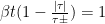 . For
. For  , this equation can be expressed as Equation 3.1.2:
 The roots can be expressed as
  . Choosing the negative sign yields the positive root that is closest to the center point
  , thereby determining the Rayleigh resolution in time domain. This result can be simplified with the Taylor series expansion of the square root in Equation 3.1.3:
 Thus, the Rayleigh resolution in time
  is approximately
  seconds. The corresponding Rayleigh range resolution is
  meters in Equation 3.1.4, with the factor of two due to the round trip of the transmitted signal.
 An important point to note is that an Arbitrary Waveform Generator (AWG) like the one in Moku:Pro generates just the real component of the chirp wave instead of its complex envelope. This leads to a divergence in the ambiguity functions of the complex envelope and sinusoid function.
The ambiguity function outlined earlier was based on the complex envelope of the received signal, however, for the sake of simplicity, the Hilbert transform was not included. For a detailed explanation of the complex envelope and related discussions, please refer to Mahafza[3].
The derivation of the ambiguity function of the real-valued sinusoidal chirp wave is challenging as it involves the Fresnel integral and manipulation of the trigonometric identities. Instead, we’ll illustrate the effect of using only the real component by examining the simple, non-modulated complex exponential wave case.
The matched filtering equation for the complex envelope of a simple non-modulated complex exponential function can be expressed as:
An important point to note is that an Arbitrary Waveform Generator (AWG) like the one in Moku:Pro generates just the real component of the chirp wave instead of its complex envelope. This leads to a divergence in the ambiguity functions of the complex envelope and sinusoid function.
The ambiguity function outlined earlier was based on the complex envelope of the received signal, however, for the sake of simplicity, the Hilbert transform was not included. For a detailed explanation of the complex envelope and related discussions, please refer to Mahafza[3].
The derivation of the ambiguity function of the real-valued sinusoidal chirp wave is challenging as it involves the Fresnel integral and manipulation of the trigonometric identities. Instead, we’ll illustrate the effect of using only the real component by examining the simple, non-modulated complex exponential wave case.
The matched filtering equation for the complex envelope of a simple non-modulated complex exponential function can be expressed as:
 Equation 3.1.5 indicates that the nulls of complex exponential ambiguity function are the combined nulls of the real part and imaginary part. The magnitudes of
  and
and  are the largest when the time offset
 τ
is zero, whereas the magnitudes of and
and  are largest at a time offset
 τ
of after period (i.e., radians), which corresponds to the nulls of the real parts
  . As a result, half the nulls of the ambiguity function are cancelled due to misalignment of real and imaginary nulls and peaks. Removing the imaginary component removes these cancellations and doubles the number of nulls.
Counterintuitively, the Rayleigh resolution is improved by approximately a factor of two for the real function compared to the full complex envelope. This illustration using the complex exponential is a general result that we can apply to our original chirp wave, as verified by simulation (Figure 2). The updated Rayleigh time resolution and range resolution values using a purely real waveform are then:
. As a result, half the nulls of the ambiguity function are cancelled due to misalignment of real and imaginary nulls and peaks. Removing the imaginary component removes these cancellations and doubles the number of nulls.
Counterintuitively, the Rayleigh resolution is improved by approximately a factor of two for the real function compared to the full complex envelope. This illustration using the complex exponential is a general result that we can apply to our original chirp wave, as verified by simulation (Figure 2). The updated Rayleigh time resolution and range resolution values using a purely real waveform are then:

 Figure 2: Comparison of the ambiguity functions of a received real-valued chirp
  and the complex envelope of the received signal (blue).
The Rayleigh resolution
and the complex envelope of the received signal (blue).
The Rayleigh resolution  determines the minimum resolution for radar in time. Figure 3 (a) shows the matched filter output of two chirps separated by exactly overlapping constructively, resulting in a flat top, which. the peak detector identifies as a single peak. In theory, when the targets are separated by any more than this, a small dip will be expected, allowing for successful separation. However, in practical applications, a small dip can be obscured by noise and it’s common to require that the filter output nominally drop to zero between pulses before two pulses can confidently be distinguished from each other. As such, this application note will focus on the demonstrations with a null-to-null width of
  .
.
 Figure 3: (a): Constructively overlapped matched filter output with a distance of
  , (b): matched filter output with
  separation nominally drops to zero between pulses. improving the chances of them being clearly distinguished in a noisy environment.
Pulse compression with Moku:Pro
In contrast to the simulation described in the introduction which used a simple on/off keyed sine wave, the simulation in this section uses a sinusoidal chirp with a large bandwidth to achieve a better Rayleigh range resolution.
Figure 4illustrates that the main lobe width of the chirp pulse is narrower compared to the sine pulse.
 Figure 4: (a-c) The same simulation as the OOK sine wave from the introduction, run with a chirp instead. (d) The matched filter output from chirp (orange) has a much smaller main lobe width than the sine wave (blue), even in the presence of overwhelming channel noise.
The Moku:Pro Multi-Instrument Mode configuration used for validation in the following sections is depicted in Figure 5. In this setup, the Arbitrary Waveform Generator (AWG) is responsible for generating two different chirp waves, with Channel B having half the bandwidth of Channel A. We use the FIR Filter Builder (FIR) to implement matched filters for the chirp waves generated by the AWG. As a result, we expect the Rayleigh resolution for Channel B output to be half that of Channel A.
Figure 4: (a-c) The same simulation as the OOK sine wave from the introduction, run with a chirp instead. (d) The matched filter output from chirp (orange) has a much smaller main lobe width than the sine wave (blue), even in the presence of overwhelming channel noise.
The Moku:Pro Multi-Instrument Mode configuration used for validation in the following sections is depicted in Figure 5. In this setup, the Arbitrary Waveform Generator (AWG) is responsible for generating two different chirp waves, with Channel B having half the bandwidth of Channel A. We use the FIR Filter Builder (FIR) to implement matched filters for the chirp waves generated by the AWG. As a result, we expect the Rayleigh resolution for Channel B output to be half that of Channel A.
 Figure 5: Moku:Pro Multi-Instrument Mode configuration used for testing and validation.
Using the AWG, we define the chirp wave using the Equation waveform type. The defining equations are shown in Equation 3.1.7:
Figure 5: Moku:Pro Multi-Instrument Mode configuration used for testing and validation.
Using the AWG, we define the chirp wave using the Equation waveform type. The defining equations are shown in Equation 3.1.7:

 Figure 6: AWG generated chirp wave, Channel A (red) is twice of the bandwidth of Channel B (blue).
The AWG generated a chirp waveform with a 200 Hz repetition rate and pulse modulation to generate chirp pulses. The equivalent bandwidth of Channel A chirp waveform is 40,000 Hz. Therefore, we expect the smallest null-to-null width 2Δ𝑡 of the combined Channel A and B waveform to be:
Figure 6: AWG generated chirp wave, Channel A (red) is twice of the bandwidth of Channel B (blue).
The AWG generated a chirp waveform with a 200 Hz repetition rate and pulse modulation to generate chirp pulses. The equivalent bandwidth of Channel A chirp waveform is 40,000 Hz. Therefore, we expect the smallest null-to-null width 2Δ𝑡 of the combined Channel A and B waveform to be:
 The FIR filter was configured as a matched filter by loading a kernel whose values were the chirp wave values, reversed in time, as per equation (3.1.10). The setup of the FIR filter is shown in Figure 7. The width of the input chirp wave and the sampling period determine the number of filter coefficients.
 The length of the AWG waveform and the FIR filter kernel is the same, and the kernel shares the same shape as the generated wave. Therefore, the equation of the FIR filter for Channel A can be written as Equation 3.1.10:

 Figure 7: FIR Filter Builder Channel A configuration.
We have now set up the transmit waveform generation and matched filtering in the AWG and FIR respectively and can examine the effects of the pulse compression. The red curve shows the output of the Channel A matched filter, the blue curve shows the output of Channel B. The blue curve has a width that is twice that of the red curve, which confirms the earlier result, proving that the time resolution of the filter output is inversely proportional to the bandwidth. The distances between the first two nulls agree with the theorem in Equation 3.1.8.
Figure 7: FIR Filter Builder Channel A configuration.
We have now set up the transmit waveform generation and matched filtering in the AWG and FIR respectively and can examine the effects of the pulse compression. The red curve shows the output of the Channel A matched filter, the blue curve shows the output of Channel B. The blue curve has a width that is twice that of the red curve, which confirms the earlier result, proving that the time resolution of the filter output is inversely proportional to the bandwidth. The distances between the first two nulls agree with the theorem in Equation 3.1.8.
 Figure 8: Pulse compression experiment based on Moku:Pro. Red curve has a bandwidth two times larger than that of the blue curve and the range resolution of the red curve is 1/2 of the blue curve.
At this point, we have completed the theory and simulation. The next step is to apply matched filtering on the chirp pulse with real noise included. The results shown in Figure 10 indicate that the matched filter performs well for large noise power (-73.98 dBm) and small signal power (-93.46 dBm).
Figure 8: Pulse compression experiment based on Moku:Pro. Red curve has a bandwidth two times larger than that of the blue curve and the range resolution of the red curve is 1/2 of the blue curve.
At this point, we have completed the theory and simulation. The next step is to apply matched filtering on the chirp pulse with real noise included. The results shown in Figure 10 indicate that the matched filter performs well for large noise power (-73.98 dBm) and small signal power (-93.46 dBm).

Figure
9: Experimental setup of the chirp matched filter in noisy environments.
 Figure 10: Power of the received signal input to the matched filter (blue) and matched filter output (red). The spike in matched filter output power clearly indicates the time of arrival of the chirp despite it being invisible to the naked eye in the received signal.
An interesting property of pulse compression is revealed by the analysis of Figure 8. The output of the matched filter for the chirp wave with a larger bandwidth has a minimum null-to-null width of 25 us and a pulse width of 5 ms. Thus, the matched filter can distinguish two overlapping reflecting chirp waves with a time distance larger than 25 us. Figures 11 and 12 display the result of the Moku:Pro experiment. Figure 11 shows the noise-free validation run, with the two overlapping chirps shown in blue and the matched filter output in red. Figure 12 shows the same experiment but with the chirps having been received on a noisy channel. In both cases, the arrival times of the two chirps are clearly distinguished from each other, and correctly found to be separated by 25 us.
Figure 10: Power of the received signal input to the matched filter (blue) and matched filter output (red). The spike in matched filter output power clearly indicates the time of arrival of the chirp despite it being invisible to the naked eye in the received signal.
An interesting property of pulse compression is revealed by the analysis of Figure 8. The output of the matched filter for the chirp wave with a larger bandwidth has a minimum null-to-null width of 25 us and a pulse width of 5 ms. Thus, the matched filter can distinguish two overlapping reflecting chirp waves with a time distance larger than 25 us. Figures 11 and 12 display the result of the Moku:Pro experiment. Figure 11 shows the noise-free validation run, with the two overlapping chirps shown in blue and the matched filter output in red. Figure 12 shows the same experiment but with the chirps having been received on a noisy channel. In both cases, the arrival times of the two chirps are clearly distinguished from each other, and correctly found to be separated by 25 us. It is worth noting that the detected time interval may exhibit a minor variation from the transmitted time separation due to the presence of non-zero side lobes in the ambiguity function.

Figure
11: Two overlapping chirp pulses with same bandwidth and time width, but a 25 us time offset (blue). The matched filter output correctly recovers the 25 us time between chirps (red).

Figure
12: Matched filter output of two overlapping chirp waves (red), compared to the received signal before filtering (blue).
Waveform triggering Digital pattern triggering, a common oscilloscope feature, involves performing logical operations on received digital signals and triggering the oscilloscope based on specific patterns. For instance, a user can set an oscilloscope to trigger only when the least significant eight bits of a digital signal are high. This feature is critical for analyzing the behavior of digital systems in various scenarios. However, in applications like chip fault injection and side-channel analysis, the signal is usually collected from a radio frequency receiver which may result in a high level of noise and low signal amplitude. In such cases, digital pattern triggering can result in numerous false alarms, giving incorrect information about the chip behavior. One solution to address the issues with digital pattern triggering is to use waveform triggering. Waveform triggering uses a matched filter to continuously compare an incoming analog signal to an expected waveform and generate a trigger event when the expected waveform is seen. Traditional oscilloscopes do not provide enough flexibility for such waveform triggering, requiring instead a dedicated “trigger box” [4]. Moku:Pro with Multi-Instrument Mode, on the other hand, allows users to deploy the FIR Filter Builder and Oscilloscope instruments simultaneously for waveform triggering and oscilloscope measurements. The waveform in Figure 13 is recreated from Beckers et al. [4] and shows power rail anomalies captured while a microprocessor encodes a data packet using Advanced Encryption Standard (AES). The detection of such an operation can then be used to launch fault injection attacks or to sample auxiliary data for later analysis. It should be noted that Beckers et al. [4] improved their results by using an envelope detector in front of the triggering algorithm. Such an operation can be completed on Moku:Pro by building a simple piece of custom logic using Moku Cloud Compile (MCC) and deploying it before the FIR instrument.
Figure
13: AES single execution pattern
If the waveform trigger will initiate sampling and recording auxiliary data, users may prefer that the trigger event as seen by the Oscilloscope occurs at the start of the matched waveform, rather than its end. In this case, extra FIR filter channels can be set up in an “all-pass” configuration, introducing a pure time delay equal to the length of the matched filter. Figure 14 demonstrates the successful generation of the trigger signal by the FIR Filter Builder, as seen on the Oscilloscope (blue). Additionally, the FIR Filter Builder has accurately delayed the unfiltered input signal, allowing users to capture the triggering waveform in its entirety for later examination. The simulation results presented in Figure 14 (a) were obtained using low-speed embedded processor waveforms with a slow sampling rate of 610 kSa/s, whereas Figure 14 (b) depicts results obtained using modern ARM processor waveforms with a sampling rate of 10 MSa/s. Despite the lower input signal SNR observed in Figure 14 (a), it is notable that the matched filter output SNR surpasses that of Figure 14 (b) due to the increased number of FIR taps and smaller noise bandwidth. To ensure accurate triggering during high-speed waveform capturing, the inclusion of pre-amplifiers is essential [4]. Moreover, the utilization of the matched output’s power (orange) to achieve improved detection accuracy can be implemented effortlessly using MCC.
Figure
14: Oscilloscope triggered by the matched filter output (blue). FIR–delayed input signal (red). Power of the matched filter output (orange).
Summary
This application note provides theoretical and empirical evidence to support the use of the matched filter as the optimal receiving filter for detection of the time of arrival of a known waveform. To verify the introduced concepts, we conducted a series of experiments using Moku:Pro Multi-Instrument Mode, the Arbitrary Waveform Generator, and the FIR Filter Builder to transmit and detect signals. Furthermore, the study explores the use of the matched filter in communication, radar pulse compression, and waveform triggering domains to highlight its efficacy in signal processing. The obtained results demonstrate the ability of Moku:Pro to reliably detect receive events in real-time, even in the presence of large noise power.References
[1] B. P. Lathi and Z. Ding, Modern digital and analog communication systems, International 4th ed. in The Oxford series in electrical and computer engineering. New York Oxford: Oxford University Press, 2010. [2] M. A. Richards, Fundamentals of radar signal processing, Third edition. New York: McGraw Hill, 2022. [3] B. R. Mahafza, Radar Systems Analysis And Design Using Matlab®, Third Edition. [4]A. Beckers, J. Balasch, B. Gierlichs, and I. Verbauwhede, “Design and Implementation of a Waveform-Matching Based Triggering System,” in
Constructive Side-Channel Analysis and Secure Design
, F.-X. Standaert and E. Oswald, Eds., in Lecture Notes in Computer Science, vol. 9689. Cham: Springer International Publishing, 2016, pp. 184–198. doi: 10.1007/978-3-319-43283-0_11.
Introduction to the matched filter
Improving the signal-to-noise ratio (SNR) in communication and radar systems is a critical requirement for enhancing detection accuracy. The matched filter is a widely employed technique to improve SNR performance when the shape of the waveform of interest is known. This contrasts with conventional filters with passbands and/or stopbands defined in the frequency domain, or the boxcar averager, which aims to eliminate time-domain elements. This application note provides a detailed exposition on the theory behind the matched filter. Additionally, we demonstrate two applications of the matched filter on Moku:Pro.Background
Derivation of the matched filter
Derivation based on continuous signals
is typically assumed to be additive white noise, with its power spectral density (PSD) being independent of frequency. Following this fundamental principle, the expected power of is constant in time, with an expected power of is constant in time, with an expected power of resulting from the multiplication of the PSD of the noise signal and the PSD of the receiving filter
The power of the received signal at time varies with the sampling time due to the non-time-invariant nature of the PSD of the transmitted signal. The PSD is given by . such that:
Therefore, the SNR at denoted can be expressed as:
To solve Equation 2.1.3 and find the condition for optimized SNR, we apply the Cauchy-Schwarz inequality. The condition for maximized SNR performance for a known transmitted signal is shown in Equation 2.1.4.
And the derived optimal filter, i.e., matched filter is given in Equation 2.1.5.
Where and is the length of the signal. The choice of leads to a filter with the shortest delay while still being casual. Additionally, the constant multiplier scales the noise and single equally and can therefore be omitted from the analysis.
Extension to a digital system
The expression in Equation 2.1.5 is the optimal filter in continuous time. To give a quantitative comparison, we will now analyze the SNR performance of the discrete time digital system. In Equation 2.2.1, the length of the matched filter is and the expected noise power is . The formula considers the the digitized channel noise , matched filtered noise , and matched filter’s impulse response
The rightmost part of in Equation 2.2.1 is the correlation of the white noise. Equation 2.2.2 indicates that the noise power has non-zero value only if . The digitized matched filter is derived from Equation 2.1.5, and the noise after the matched filtering is shown in Equation 2.2.3:
The peak power of the matched filter output is given by Equation 2.2.4. The matched filter output peak power is the square of the energy of the transmitted pulse because the matched filter impulse response is the time-reverse transmitted pulse
Therefore, the SNR at the peak of the output signal becomes the formula in Equation 2.2.5. Note that the power of the transmitted signal is given by and the noise power is given by
The SNR improvement rate accords with the SNR increase in the simulation in the Introduction section. That simulation showed a 21.75 dB SNR improvement with a 150-sample filter, and the quantitative analysis gives enhancement.
Applications of the matched filter
In this section, we introduce and explain two applications of the matched filter: radar distance sensing (pulse compression) and waveform triggering.
Radar pulse compression
In the first example, we will examine radar pulse compression. In a radar system, a transmitter emits a burst of radio waves toward a target. The radar receiver then listens for the return echoes reflected by the target. The time of flight, or range delay, allows us to calculate the distance to the target. This application bears resemblance to the communication example shown in Figure 1, as both radar and communication systems are designed to detect signals in noisy receiving environments. A conventional radar lacking a matched filter requires a high transmitting power to be effectively implemented, and its range resolution is significantly restricted by the length of the transmitting pulse. To address this issue, a matched filter can be used to compress the received pulse in time. A narrow pulse output from the filter gives the best spatial resolution, while the actual transmitted signal can remain broad to increase transmitted energy and therefore boost SNR without requiring high power. Specifically, a chirp (sine wave of linearly increasing frequency) is often used as the transmitted signal due to its narrow autocorrelation and relative simplicity of generation.Theory and derivation
Richards
[2] derived Equation 3.1.1, which specifies the ambiguity function of the complex envelope of chirp waves, with
The range resolution of the radar is determined by the Rayleigh resolution, which is the distance between the peak and the first null point. The peak of is observed at , and the first null occurs when the argument of the numerator equals , i.e., when . For , this equation can be expressed as Equation 3.1.2:
The roots can be expressed as . Choosing the negative sign yields the positive root that is closest to the center point , thereby determining the Rayleigh resolution in time domain. This result can be simplified with the Taylor series expansion of the square root in Equation 3.1.3:
Thus, the Rayleigh resolution in time is approximately seconds. The corresponding Rayleigh range resolution is meters in Equation 3.1.4, with the factor of two due to the round trip of the transmitted signal.
An important point to note is that an Arbitrary Waveform Generator (AWG) like the one in Moku:Pro generates just the real component of the chirp wave instead of its complex envelope. This leads to a divergence in the ambiguity functions of the complex envelope and sinusoid function.
The ambiguity function outlined earlier was based on the complex envelope of the received signal, however, for the sake of simplicity, the Hilbert transform was not included. For a detailed explanation of the complex envelope and related discussions, please refer to Mahafza[3].
The derivation of the ambiguity function of the real-valued sinusoidal chirp wave is challenging as it involves the Fresnel integral and manipulation of the trigonometric identities. Instead, we’ll illustrate the effect of using only the real component by examining the simple, non-modulated complex exponential wave case.
The matched filtering equation for the complex envelope of a simple non-modulated complex exponential function can be expressed as:
Equation 3.1.5 indicates that the nulls of complex exponential ambiguity function are the combined nulls of the real part and imaginary part. The magnitudes of and are the largest when the time offset τ
is zero, whereas the magnitudes of and are largest at a time offset τ
of after period (i.e., radians), which corresponds to the nulls of the real parts . As a result, half the nulls of the ambiguity function are cancelled due to misalignment of real and imaginary nulls and peaks. Removing the imaginary component removes these cancellations and doubles the number of nulls.
Counterintuitively, the Rayleigh resolution is improved by approximately a factor of two for the real function compared to the full complex envelope. This illustration using the complex exponential is a general result that we can apply to our original chirp wave, as verified by simulation (Figure 2). The updated Rayleigh time resolution and range resolution values using a purely real waveform are then:
Figure 2: Comparison of the ambiguity functions of a received real-valued chirp and the complex envelope of the received signal (blue).
The Rayleigh resolution determines the minimum resolution for radar in time. Figure 3 (a) shows the matched filter output of two chirps separated by exactly overlapping constructively, resulting in a flat top, which. the peak detector identifies as a single peak. In theory, when the targets are separated by any more than this, a small dip will be expected, allowing for successful separation. However, in practical applications, a small dip can be obscured by noise and it’s common to require that the filter output nominally drop to zero between pulses before two pulses can confidently be distinguished from each other. As such, this application note will focus on the demonstrations with a null-to-null width of .
Figure 3: (a): Constructively overlapped matched filter output with a distance of , (b): matched filter output with separation nominally drops to zero between pulses. improving the chances of them being clearly distinguished in a noisy environment.
Pulse compression with Moku:Pro
In contrast to the simulation described in the introduction which used a simple on/off keyed sine wave, the simulation in this section uses a sinusoidal chirp with a large bandwidth to achieve a better Rayleigh range resolution.
Figure 4illustrates that the main lobe width of the chirp pulse is narrower compared to the sine pulse.
Figure 4: (a-c) The same simulation as the OOK sine wave from the introduction, run with a chirp instead. (d) The matched filter output from chirp (orange) has a much smaller main lobe width than the sine wave (blue), even in the presence of overwhelming channel noise.
The Moku:Pro Multi-instrument Mode configuration used for validation in the following sections is depicted in Figure 5. In this setup, the Arbitrary Waveform Generator (AWG) is responsible for generating two different chirp waves, with Channel B having half the bandwidth of Channel A. We use the FIR Filter Builder (FIR) to implement matched filters for the chirp waves generated by the AWG. As a result, we expect the Rayleigh resolution for Channel B output to be half that of Channel A.
Figure 5: Moku:Pro Multi-instrument Mode configuration used for testing and validation.
Using the AWG, we define the chirp wave using the Equation waveform type. The defining equations are shown in Equation 3.1.7:
Figure 6: AWG generated chirp wave, Channel A (red) is twice of the bandwidth of Channel B (blue).
The AWG generated a chirp waveform with a 200 Hz repetition rate and pulse modulation to generate chirp pulses. The equivalent bandwidth of Channel A chirp waveform is 40,000 Hz. Therefore, we expect the smallest null-to-null width 2Δ𝑡 of the combined Channel A and B waveform to be:
The FIR filter was configured as a matched filter by loading a kernel whose values were the chirp wave values, reversed in time, as per equation (3.1.10). The setup of the FIR filter is shown in Figure 7. The width of the input chirp wave and the sampling period determine the number of filter coefficients.
The length of the AWG waveform and the FIR filter kernel is the same, and the kernel shares the same shape as the generated wave. Therefore, the equation of the FIR filter for Channel A can be written as Equation 3.1.10:
Figure 7: FIR Filter Builder Channel A configuration.
We have now set up the transmit waveform generation and matched filtering in the AWG and FIR respectively and can examine the effects of the pulse compression. The red curve shows the output of the Channel A matched filter, the blue curve shows the output of Channel B. The blue curve has a width that is twice that of the red curve, which confirms the earlier result, proving that the time resolution of the filter output is inversely proportional to the bandwidth. The distances between the first two nulls agree with the theorem in Equation 3.1.8.
Figure 8: Pulse compression experiment based on Moku:Pro. Red curve has a bandwidth two times larger than that of the blue curve and the range resolution of the red curve is 1/2 of the blue curve.
At this point, we have completed the theory and simulation. The next step is to apply matched filtering on the chirp pulse with real noise included. The results shown in Figure 10 indicate that the matched filter performs well for large noise power (-73.98 dBm) and small signal power (-93.46 dBm).
Figure
9: Experimental setup of the chirp matched filter in noisy environments.
Figure 10: Power of the received signal input to the matched filter (blue) and matched filter output (red). The spike in matched filter output power clearly indicates the time of arrival of the chirp despite it being invisible to the naked eye in the received signal.
An interesting property of pulse compression is revealed by the analysis of Figure 8. The output of the matched filter for the chirp wave with a larger bandwidth has a minimum null-to-null width of 25 us and a pulse width of 5 ms. Thus, the matched filter can distinguish two overlapping reflecting chirp waves with a time distance larger than 25 us. Figures 11 and 12 display the result of the Moku:Pro experiment. Figure 11 shows the noise-free validation run, with the two overlapping chirps shown in blue and the matched filter output in red. Figure 12 shows the same experiment but with the chirps having been received on a noisy channel. In both cases, the arrival times of the two chirps are clearly distinguished from each other, and correctly found to be separated by 25 us. It is worth noting that the detected time interval may exhibit a minor variation from the transmitted time separation due to the presence of non-zero side lobes in the ambiguity function.
Figure
11: Two overlapping chirp pulses with same bandwidth and time width, but a 25 us time offset (blue). The matched filter output correctly recovers the 25 us time between chirps (red).
Figure
12: Matched filter output of two overlapping chirp waves (red), compared to the received signal before filtering (blue).
Waveform triggering Digital pattern triggering, a common oscilloscope feature, involves performing logical operations on received digital signals and triggering the oscilloscope based on specific patterns. For instance, a user can set an oscilloscope to trigger only when the least significant eight bits of a digital signal are high. This feature is critical for analyzing the behavior of digital systems in various scenarios. However, in applications like chip fault injection and side-channel analysis, the signal is usually collected from a radio frequency receiver which may result in a high level of noise and low signal amplitude. In such cases, digital pattern triggering can result in numerous false alarms, giving incorrect information about the chip behavior. One solution to address the issues with digital pattern triggering is to use waveform triggering. Waveform triggering uses a matched filter to continuously compare an incoming analog signal to an expected waveform and generate a trigger event when the expected waveform is seen. Traditional oscilloscopes do not provide enough flexibility for such waveform triggering, requiring instead a dedicated “trigger box” [4]. Moku:Pro with Multi-instrument Mode, on the other hand, allows users to deploy the FIR Filter Builder and Oscilloscope instruments simultaneously for waveform triggering and oscilloscope measurements. The waveform in Figure 13 is recreated from Beckers et al. [4] and shows power rail anomalies captured while a microprocessor encodes a data packet using Advanced Encryption Standard (AES). The detection of such an operation can then be used to launch fault injection attacks or to sample auxiliary data for later analysis. It should be noted that Beckers et al. [4] improved their results by using an envelope detector in front of the triggering algorithm. Such an operation can be completed on Moku:Pro by building a simple piece of custom logic using Moku Cloud Compile (MCC) and deploying it before the FIR instrument.
Figure
13: AES single execution pattern
If the waveform trigger will initiate sampling and recording auxiliary data, users may prefer that the trigger event as seen by the Oscilloscope occurs at the start of the matched waveform, rather than its end. In this case, extra FIR filter channels can be set up in an “all-pass” configuration, introducing a pure time delay equal to the length of the matched filter. Figure 14 demonstrates the successful generation of the trigger signal by the FIR Filter Builder, as seen on the Oscilloscope (blue). Additionally, the FIR Filter Builder has accurately delayed the unfiltered input signal, allowing users to capture the triggering waveform in its entirety for later examination. The simulation results presented in Figure 14 (a) were obtained using low-speed embedded processor waveforms with a slow sampling rate of 610 kSa/s, whereas Figure 14 (b) depicts results obtained using modern ARM processor waveforms with a sampling rate of 10 MSa/s. Despite the lower input signal SNR observed in Figure 14 (a), it is notable that the matched filter output SNR surpasses that of Figure 14 (b) due to the increased number of FIR taps and smaller noise bandwidth. To ensure accurate triggering during high-speed waveform capturing, the inclusion of pre-amplifiers is essential [4]. Moreover, the utilization of the matched output’s power (orange) to achieve improved detection accuracy can be implemented effortlessly using MCC.
Figure
14: Oscilloscope triggered by the matched filter output (blue). FIR–delayed input signal (red). Power of the matched filter output (orange).
Summary
This application note provides theoretical and empirical evidence to support the use of the matched filter as the optimal receiving filter for detection of the time of arrival of a known waveform. To verify the introduced concepts, we conducted a series of experiments using Moku:Pro Multi-instrument Mode, the Arbitrary Waveform Generator, and the FIR Filter Builder to transmit and detect signals. Furthermore, the study explores the use of the matched filter in communication, radar pulse compression, and waveform triggering domains to highlight its efficacy in signal processing. The obtained results demonstrate the ability of Moku:Pro to reliably detect receive events in real-time, even in the presence of large noise power.References
[1] B. P. Lathi and Z. Ding, Modern digital and analog communication systems, International 4th ed. in The Oxford series in electrical and computer engineering. New York Oxford: Oxford University Press, 2010. [2] M. A. Richards, Fundamentals of radar signal processing, Third edition. New York: McGraw Hill, 2022. [3] B. R. Mahafza, Radar Systems Analysis And Design Using Matlab®, Third Edition. [4]A. Beckers, J. Balasch, B. Gierlichs, and I. Verbauwhede, “Design and Implementation of a Waveform-Matching Based Triggering System,” in
Constructive Side-Channel Analysis and Secure Design
, F.-X. Standaert and E. Oswald, Eds., in Lecture Notes in Computer Science, vol. 9689. Cham: Springer International Publishing, 2016, pp. 184–198. doi: 10.1007/978-3-319-43283-0_11.