The Moku Time & Frequency Analyzer from Liquid Instruments is a flexible and powerful instrument, functioning as a time tagger, frequency counter, event counter, event timer, and more. It can run on its own or in Multi-Instrument Mode alongside any other Moku instruments. For example, it’s easy to deploy it alongside the Moku Oscilloscope to view and debug the timing edges or the Moku PID Controller for closed-loop stabilization of count rates.
Running the Time & Frequency Analyzer on a Moku device means relying on the platform’s high-speed sampling front end, rather than bespoke time-to-digital conversion frontends used on some dedicated timing devices. A sampled architecture provides lower dead time and more flexibility, but can require more precise preconditioning of the input signal.
In this application note, we examine the Time & Frequency Analyzer’s interpolation modes and noise characteristics to understand how to get the best possible measurement accuracy in your experiment.
Instrument basics
The Time & Frequency Analyzer instrument works very simply by recording the time of arrival of a series of edges. The edge detectors at the front of the Time & Frequency Analyzer can be configured with the edge polarity (i.e., rising or falling), and the voltage threshold at which the edge is said to have occurred. The edge detectors take as input samples from the Moku analog to digital converters (ADCs), and are able to provide sub-sample estimates of edge arrival time by interpolation (see more details below).
The timestamps from the edge detectors can be logged directly, or they can be used as input to one or more interval analyzers. The interval analyzers compute statistics on the difference between timestamps. For example, the period between events can be used to calculate the frequency in a frequency counter application.
Even though you will most likely interact with the interval analyzers and the statistics they produce, it’s important to know that it’s the edge detectors that are responsible for producing timestamps accurate to a few tens of picoseconds. The rest of this note will examine in detail how they’re able to achieve this.
Jitter, resolution, and accuracy
The performance of the Moku Time & Frequency Analyzer is characterized by three related parameters: measurement jitter, measurement accuracy, and digital resolution (Figure 1).
What is jitter?
Jitter is a measure of how much variation you would expect in repeated measurements of the same edge arrival time. The accuracy is a measure of how close any single measurement is to the true value (sometimes explicitly called the “single shot” accuracy). The jitter is usually given as the standard deviation of the distribution of a large number of repeated measurements. This makes the jitter independent of bias (i.e., non-zero mean) and while not strictly required, it’s often implicitly assumed that the distribution is Gaussian. The accuracy may be given as an RMS error or mean-absolute error. In the specific case of a non-biased measurement, the RMS accuracy and the jitter are the same. Note that in this formulation, as bias grows, accuracy degrades but jitter does not.
Resolution, or more correctly the digital resolution, is the smallest difference between two measurements that the instrument can report. As long as this number is substantially smaller than the jitter (or accuracy), then resolution is not a performance measure. It’s easy to add more and more digital resolution, but if the jitter is not improved, then all those extra digits only contain noise and do not give any more information about the signal.
The Time & Frequency Analyzer has a digital resolution generally around 20x finer than the jitter, and the measurement is not biased. As such, digital resolution is not a performance limitation, and accuracy and jitter measures are the same.

Figure 1: The jitter, accuracy, and resolution of a timing histogram. Jitter is the standard deviation of the measurement distribution and is independent of bias. Accuracy is the RMS value of the measurements. Resolution is the smallest representable change in measurement value and is rarely the limiting factor for performance. For the purposes of illustration, the histogram is biased by more than would be typical for a real instrument.
Interpolation modes
The Moku Time & Frequency Analyzer uses a sampled front end. Moku:Pro samples at 1.25GSa/s by default, giving a period of 800 picoseconds. Without any further processing, this 800-picosecond value would be the digital resolution and, being higher than the underlying jitter, would be the performance limiting factor. The Time & Frequency Analyzer can improve on this by using an interpolation algorithm to get a sub-sample estimate of the point at which the signal crossed the threshold. The instrument’s linear interpolation works very well for a wide variety of signals, and is able to improve timing performance by around 100x compared to no interpolation.
Linear interpolation makes one very important assumption: That the rising edge is linear between the sample points either side of the threshold crossing. This introduces two related requirements on the rise time of your signal (assuming a rising edge trigger):
- That the rising edge is slow enough compared to the sample rate that there are several samples on the edge itself, and
- That the rising edge is slow enough compared to the bandwidth of the Moku that the step response of the Moku front end isn’t limiting the rise time.
This second point ensures that the signal is rising approximately linearly as it crosses the threshold, as opposed to being in a nonlinear portion of an exponential convergence. It also means that for best results, you should try to choose a threshold value where the signal is approximately linear. For example, if you’re looking at the timing of a sine wave in a frequency counter application, the threshold should be set to the mean value of the sine wave (usually the zero crossing).
An example is shown below in Figure 2 for a step input with three different edge speeds. For the fastest edge (left), the actual signal (dark) can move by as much as a whole sample period without affecting the values actually sampled by the ADC, and therefore without changing the interpolated rising edge (light blue). On the other hand, with an edge rate slow enough that there are always sample points on the edge either side of the threshold (right), the actual and interpolated edges cross the threshold at exactly the same point and the edge position is recorded perfectly. In the transition region between the two extremes, only one or two sample points are on the rising edge and therefore the interpolated value is biased towards the point halfway between sample times, but not limited to it.

Figure 2: Edge rate impacts ADC sampling accuracy, with fast edges allowing signal shifts and slow edges ensuring precise threshold alignment, while transition regions introduce interpolation bias.
Another way to look at this is to examine how the distribution of edge times changes as the edge rate increases. For slow edges, the distribution of interpolated times matches the real values very closely. As the edge rate speeds up, the distribution starts to bias towards the point halfway between samples (as seen in the left-most illustration above). This simple simulation starts to show bias as the number of sample points per edge drops down below two.
As we can see, the Time & Frequency Analyzer linear interpolation is able to capture edge times that are jitter-limited (rather than resolution limited), so long as the assumption that the rising edge is linear around the threshold holds. Figure 3 shows that as the edge rate increases past a point, the measurement gets worse. The distribution of edge times biases towards multiples of the sample period, the accuracy degrades, and the jitter begins to depend on the actual value of the edge arrival time relative to the sample times.
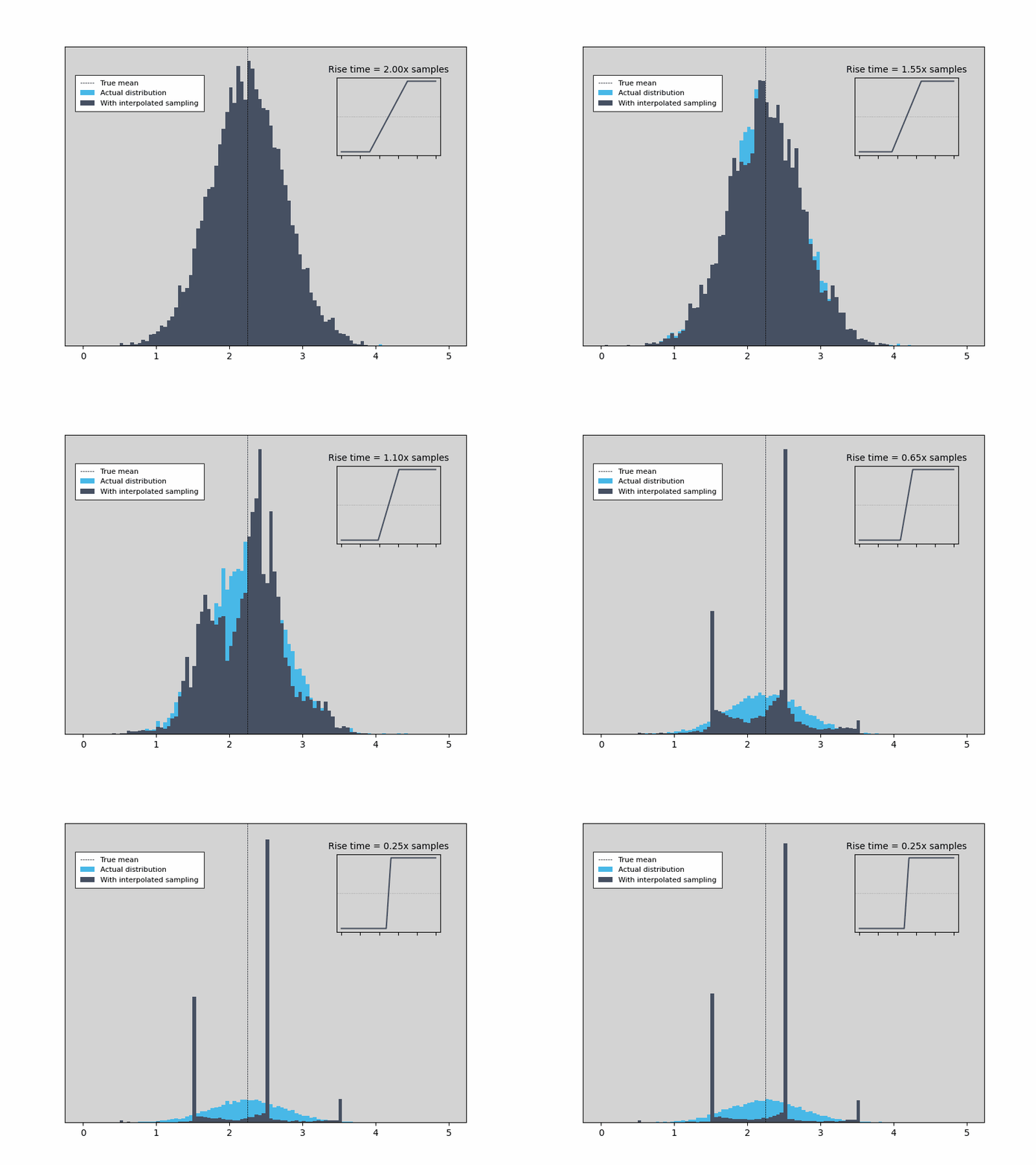
Figure 3: As the edge rate increases past a point, the measurement gets worse.
Optimizing your measurement
If the interpolation algorithm is required to get high resolution, and works best with slower edge rates, why wouldn’t you just continue to slow the edge down indefinitely? All Time & Frequency Analyzer instruments have an intrinsic timing jitter, based on the performance of the internal oscillators and clocking infrastructure, and also intrinsic amplitude noise based on the performance of the components in the analog signal chain. As the edge rate gets slower, the amplitude noise moves the threshold crossing point in time by a greater amount.
In Figure 4, the three signals have the same amount of amplitude noise, and the histogram of the threshold-crossing location is plotted in blue below. When the edge rate is fast, the amplitude noise doesn’t cause a spread of the measurement distribution at all, while slower edge rates cause timing jitter to be seen due to coupling of that amplitude noise.
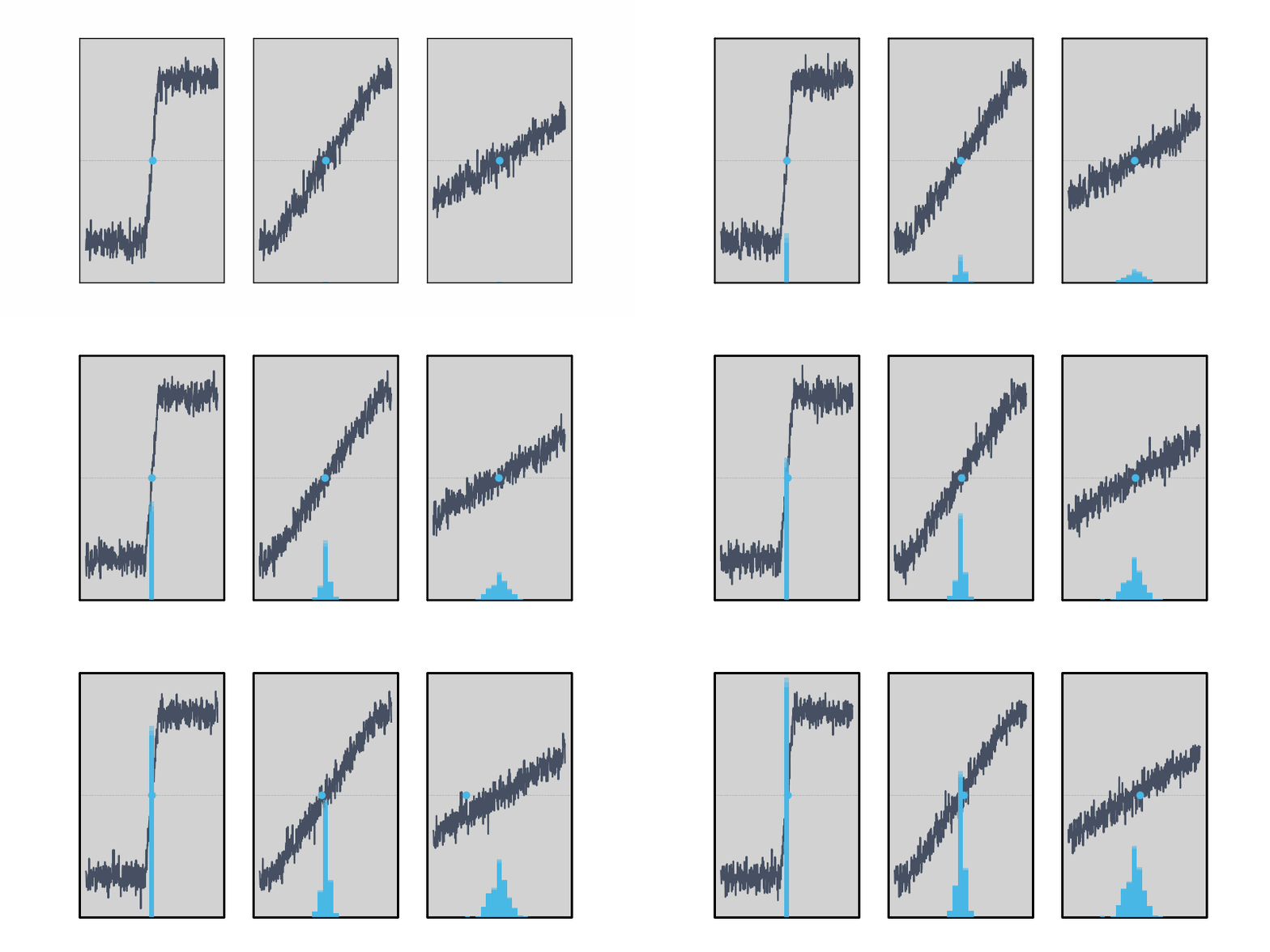
Figure 4: The rise time affects how much the amplitude noise of a signal couples in to the timing. For fast edges, the threshold crossing doesn’t move at all.
We now have two competing requirements: The edge must be fast to couple the minimum amount of amplitude noise into the threshold crossing time, and slow to preserve the assumption of linearity that’s required to interpolate between points on the Moku Time & Frequency Analyzer’s sampled front end. Getting the best possible measurement then requires a “goldilocks” edge rate: not too fast and not too slow. This is characterized for each Moku hardware platform and given in the Moku Time & Frequency Analyzer specification sheet as the “optimum” rise time. For example, Moku:Pro has an optimum rise time of 6 ns, or around 7.5 sample periods — enough to guarantee that the edge is sampled in the linear region around the trigger point.
If you don’t have direct control over the edge rate of your signal, the best way to meet the optimum rise time is to put it through a low-pass filter before it goes into the Moku. The conversion between rise time and filter bandwidth is approximately BW = 0.35 / rise (assuming a first-order Butterworth filter). For example, to meet the optimum rise time for Moku:Pro of 6 ns, a 60 MHz low-pass filter is recommended.
It’s natural to wonder whether the filter changes the timing characteristics of the signal that you’re trying to measure. It does, in that it introduces group delay on the signal; but it’s the same delay for all edges. Given that the Moku time stamps are relative to an arbitrary origin time, moving all measurements forward or back by the same amount has no overall effect. Another way to think of this is like using a slightly longer cable — it’s important that all inputs are matched, but not what the absolute length of the cables are.
Conclusion
The Moku Time & Frequency Analyzer is a powerful tool for the analysis of event times and their statistics. The Time & Frequency Analyzer shares its analog front end with the rest of the Moku suite of software-defined instrumentation and, along with flexibility, this sampled architecture brings a greater dependence on edge times when optimizing your measurement. The signal can:
- Not be interpolated at all: This is robust but limits the performance of the instrument to the sample rate (800ps on Moku:Pro).
- Rise too quickly: The one-shot measurement accuracy may be similar to the optimal case, but the value becomes biased.
- Rise too slowly: The amplitude noise of the analog frontend couples into the threshold crossing time and introduces extra timing jitter.
The good news is that it’s easy to condition your edge for excellent Time & Frequency Analyzer performance. The Moku specification sheet gives optimal rise time values that minimize jitter while preventing bias, and these rise times can be met by the simple expedient of adding a low-pass filter in series with your signal.
Questions?
Get answers to FAQs in our Knowledge Base
If you have a question about a device feature or instrument function, check out our extensive Knowledge Base to find the answers you’re looking for. You can also quickly see popular articles and refine your search by product or topic.
Join our User Forum to stay connected
Want to request a new feature? Have a support tip to share? From use case examples to new feature announcements and more, the User Forum is your one-stop shop for product updates, as well as connection to Liquid Instruments and our global user community.
