



In Part 1 of this white paper, we introduce 2-level quantum systems known as qubits, which are used in various applications ranging from quantum computation to magnetic field sensing. We examine a few examples of how qubits are physically implemented, as well as the structure of a generic two-level quantum system.
In Part 2, we introduce the graphical representation of qubit states known as the Bloch sphere. We also use this model to demonstrate how common pulse sequences such as Rabi, Ramsey, and CPMG can be implemented on reconfigurable hardware such as Moku to extract key information from these qubits.
Download and read the entire white paper here.
What is a qubit?
A quantum bit, or qubit, is a basic building block of quantum computing, communication, and sensing. Similar to a classical bit, a qubit is a physical system that can inhabit two distinct, quantized states corresponding to classical 0 and 1. We represent these quantum states as ∣0⟩ and ∣1⟩, consistent with most work in the field. Like how in a transistor 0 and 1 represent the presence or absence of current flow, the state of a qubit corresponds to some physically measurable parameter, such as electron spin or atomic energy level. As we will see in the next sections, their quantum nature means that qubits can also exist in superposition of these two states. The basic requirements for a useful qubit are [1]:
- Initialization, meaning the qubits can be set or reset to the 0 state.
- Coherent manipulation, the use of microwave or laser pulses to drive the qubit state.
- Readout, where the state of the qubit is probed and delivered to the end user.
Note that even while existing in a superposition state, qubits can only ever return 0 or 1 during readout, meaning that many repetitions of a given experiment are required to determine the full picture of the state. This will be examined further when discussing pulse sequences in the final section.
Many competing qubit systems exist, each with their own advantages and disadvantages. While it is outside the scope of this work to discuss the merits of specific qubit archetypes, a few examples of physical implementations and the physical quantity include:
Superconducting transmon qubits, formed by patterning superconducting Josephson junctions on a substrate. In these systems, the ∣0⟩ and ∣1⟩ states correspond to the two lowest energy levels of a nonlinear oscillator defined by the interplay of superconducting current, charge, and phase across the junction.
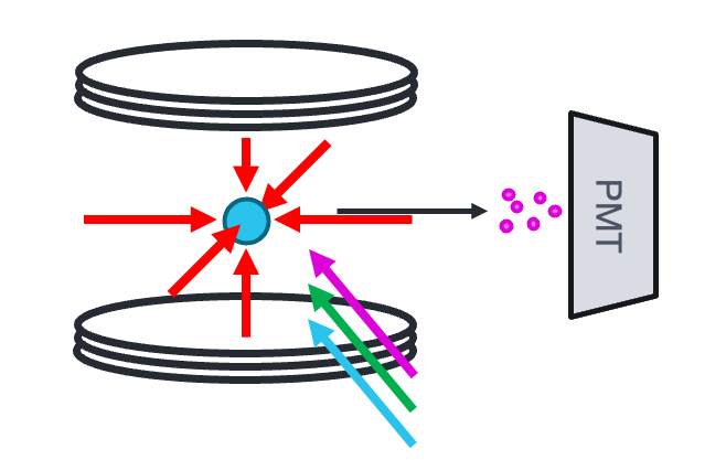
Neutral atoms, held in place by a combination of laser beams and magnetic fields. The qubit states are two carefully selected atomic energy levels, typically defined by either Zeeman splitting in a magnetic field or hyperfine interactions between the nucleus and valence electrons. An example can be seen in Fig 1.
Solid-state qubits, such as nitrogen-vacancy (NV) centers in diamond, created by introducing electron-donating nitrogen atoms near lattice vacancies. When placed in a DC magnetic field, multiple electron spin states are split via the Zeeman effect, with two levels selected to serve as ∣0⟩ and ∣1⟩.
In the next section, we introduce the mathematical description of a qubit system.
The two-level quantum system
To build intuition for how qubits behave, we start with a so-called two-level quantum system. As mentioned, this could be many things: the spin of an electron, two hyperfine states of an ion, or the two lowest energy levels of a superconducting circuit. Physically, these systems are very different, but they can all be described by the same simple model. Using bra-ket notation, common in quantum physics, we label the two energy levels as:
|0⟩: the lower energy state (ground state)
|1⟩: the higher energy state (excited state)
Superposition states are written as a linear combination of |0⟩ and |1⟩, with |𝜓⟩ representing this superposition state. To quantify the degree of mixing between the two states, we also introduce amplitudes α and ꞵ. Put together, any possible state of two-level system can be written as:
\(| \psi \rangle = \alpha | 0 \rangle + \beta | 1 \rangle \) (1)
The amplitudes obey the normalization condition \(| \alpha |^2 + | \beta |^2 = 1\), with \(| \alpha |^2 \) and \(| \beta |^2 \) representing the probability to find the qubit in that state. Setting α = 1 and β = 0 would imply that the system exists fully in the classical 0 state, whereas \(\alpha = \beta = 1/\sqrt{2}\) represents a 50/50 superposition of the two states – equally likely for the system to be measured in either state.
Note that α and β can be real or complex, and the relative phase between them plays a crucial role in quantum interference and time evolution. This form describes what is known as a pure state, but as we’ll see, interaction with the environment can quickly cause the system to become mixed.
In the next section we introduce the Hamiltonian and see how it encodes the energy level information.
The system Hamiltonian
In a two-level quantum system, the energy difference between these states is typically written in terms of frequency, ℏω, where ℏ is the reduced Planck’s constant and ω is the frequency of the EM radiation that is absorbed or emitted to transition between the two energy levels. The dynamics of this system are governed by a very simple Hamiltonian, given in Eq. 2. In quantum mechanics, an operator (represented by a caret ^ above the symbol) is a mathematical object that acts on a quantum state to change or measure something about it such as its energy, position, or spin. In the Hamiltonian’s case, it is the total energy of the system.
\(\widehat{H} = \frac{-1}{2} ℏ ω_0 \widehat{σ}_z \) (2)
Here, \(\widehat{σ}_z\) is one of the Pauli matrices. Originally introduced to describe electron spin, Pauli matrices now serve as a general-purpose basis for describing any two-level quantum system. In this case, z defines the quantization axis, or the axis along which the two energy levels ∣0⟩ and ∣1⟩ are split. It encodes the fact that state ∣1⟩ has higher energy than ∣0⟩.
The action of \(\widehat{σ}_z\) on the two basis states is:
\(\widehat{σ}_z |0 \rangle = -|0\rangle, \widehat{σ}_z |1\rangle = | 1\rangle \)
This reflects the energy difference between the two levels, with the minus sign indicating that the two states lie on opposite sides of the quantization axis. In spin-based systems (like NMR or electron spin qubits), the quantization axis is usually set by an external magnetic field, and the energy levels split along that axis. In atomic and superconducting qubits, it’s defined by other system-specific factors.
Let’s now examine how the system evolves in time.
Time evolution
Quantum systems are dynamic, but so far, we’ve only examined how a system’s state is defined at a single point in time. We substitute the state vector |𝜓⟩ for a time-dependent one |𝜓(t)⟩ and introduce the famous Schrödinger equation, which describes the evolution of quantum systems over time, given their Hamiltonian:
\(i\hbar\frac{\partial}{\partial t} | \psi(t)\rangle=\widehat{H} | \psi(t)\rangle\) (3)
Essentially, applying the Hamiltonian operator gives us information about how the state vector |𝜓(t)⟩ evolves. Revisiting our two-level Hamiltonian (Eq 2), we note that the value t does not appear anywhere within it, meaning that our energy levels are fixed in time. When this is the case, the Schrödinger equation has a simple solution describing how the state evolves from time \(i\hbar\frac{\partial}{\partial t}\left|\Psi(t)\right>=\widehat{H}\left|\Psi(t)\right>\) to a later time t [2]:
\(| \psi(t) \rangle = e^{\frac{- i \widehat{H} t}{\hbar}} | \psi(0) \rangle\)
For our specific system:
\(| \psi(t) \rangle = e^{\frac{- i \omega_0 t \widehat{\sigma}_z }{2}} | \psi(0) \rangle\)
While the Hamiltonian has no explicit time dependence, the system evolves in time because these two states have different energies. Crucially, this evolution happens regardless of the physical system: whether the energy splitting is due to a magnetic field, hyperfine structure, or an engineered quantum circuit. This makes our equation universal for any two-state quantum system.
Let’s look at how this plays out for two different initial states. First, we’ll start in the ground state ∣0⟩:
\(| \psi(0) \rangle = | 0 \rangle\)
Applying the time evolution operator:
\(| \psi(0) \rangle = e^{\frac{i \omega_0 t}{2}} | 0 \rangle\)
This is just a global phase change over time, which has no observable effect when we read out the qubit (recall that we only ever observe ∣0⟩ or ∣1⟩, with probability equal to the modulus squared of each state’s coefficient).
Now we examine the case where we start in an equal superposition:
\(| \psi(0) \rangle = \frac{1}{\sqrt{2}} \left( |0 \rangle + | 1 \rangle \right) \)
Now apply the time evolution operator to each component:
\(| \psi(t) \rangle = \frac{1}{\sqrt{2}} e^{\frac{- i \omega_0 t \widehat{\sigma}_z }{2}} \left( |0 \rangle + | 1 \rangle \right) = \frac{1}{\sqrt{2}} e^{\frac{i \omega_0 t}{2}} |0 \rangle + \frac{1}{\sqrt{2}}e^{\frac{-i \omega_0 t}{2}} |1 \rangle\)
This can also be written as:
\(| \psi(t) \rangle = \frac{e^{\frac{-i \omega_0 t}{2}}}{\sqrt{2}} \left( |0 \rangle + e^{i \omega_0 t}| 1 \rangle \right) \)
Again, the actual value of the global phase \(e^\frac{-i \omega_0 t}{2}\) has no physical relevance, and the probability of reading out a ∣0⟩ or a ∣1⟩ doesn’t change over time. Importantly, though, the relative phase of the ∣0⟩ and ∣1⟩ states evolves in time at frequency \(\omega_0 \).
In this first part of the white paper, we’ve given an overview of the two-level quantum system. In Part 2, we will visualize this phase difference and see the consequences, as well as discuss protocols and hardware implementation.
References and Footnotes
[1] DiVincenzo, David. The Physical Implementation of Quantum Computation. https://doi.org/10.48550/arXiv.quant-ph/0002077
[2] For a more formal derivation of this solution, including how time evolution operators arise from the Schrödinger equation, we refer the reader to any standard quantum mechanics textbook. Griffiths’ Introduction to Quantum Mechanics is particularly accessible and widely beloved, with good reason.