Mastering the Moku Time & Frequency Analyzer

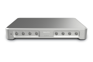
Now available with the Moku Version 3.2 software update, we’re thrilled to introduce our 14th instrument, the Time & Frequency Analyzer.

From biological imaging to quantum optics, Moku users have consistently requested the ability to characterize the number and rate of occurrence of transient events in their time-domain signals. With the introduction of the Time & Frequency Analyzer, sub-ns-resolution measurements are now available on all Moku devices. In this white paper, we introduce the concept of time interval measurement and explore various applications.

How does the Time & Frequency Analyzer capture events, intervals, and measurements?

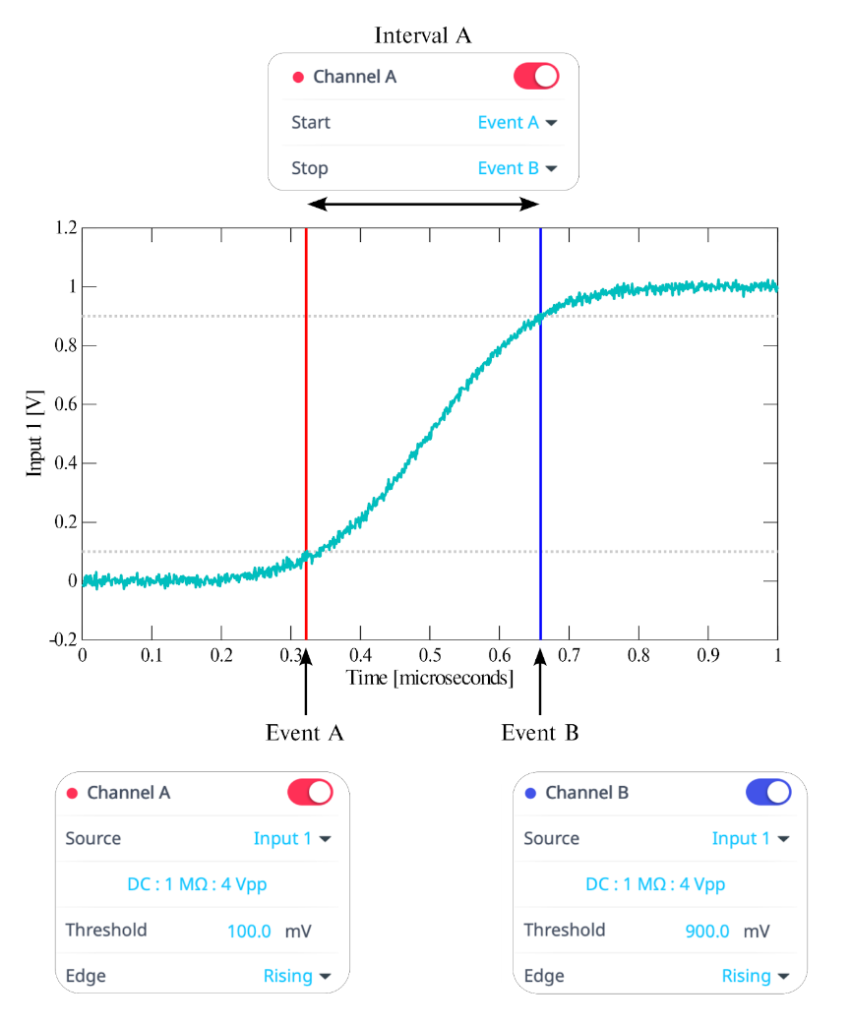
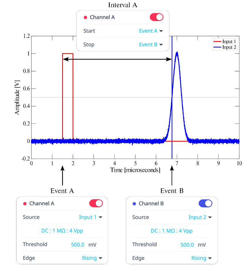
Two fundamental concepts underpin Time & Frequency Analyzer measurements, events and intervals. An event occurs when an input signal crosses a fixed threshold level. This crossing may be positive-going, negative-going, or defined to include both crossings, such that a pulse would be recorded as an event but a step would not.

An interval is the time that elapses between two events. Any pair of valid events may be used. There is no requirement that the two events come from the same signal, and there is also no requirement that the events be different (in which case, the interval between successive events of the same type would be measured). Figure 1 illustrates a basic measurement configuration.

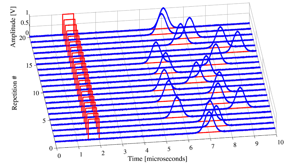
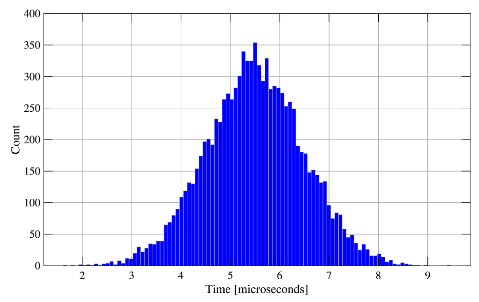
TFA measurement — Figure 1: The Time & Frequency Analyzer operates using events and intervals. This example demonstrates how to measure the rise time of an input signal via definition of two rising-edge events, Event A with a threshold of 0.1 V and Event B with a threshold of 0.9 V. Interval A is defined as the time that elapses between Event A and Event B.

The instrument’s measurement process is continuous and results are aggregated, allowing the user to construct a histogram of individual measurements (see Figures 2 and 3) and compute the statistics of both events (count, rate) and intervals (count, mean, min, max) over time. Alternatively, the desired metrics may be evaluated over a window of finite duration, defined either internally or via an external gating signal. This concept is explained further in the Applications section below.

Figure 2: Events need not be defined on the same input channel. The above image indicates how one might configure a typical stimulus-response experiment. The generation of the stimulus is indicated by the arrival of a pulse (Input 1, red), which triggers Event A. The resulting response (Input 2, blue) is recorded as Event B. Interval A measures the elapsed time between Event A and Event B (i.e., between the stimulus and the response).

Finally, the Time & Frequency Analyzer allows the user to output the current interval, event count, or interval count as an analog voltage suitable for integration into a wider experimental setup.

Figure 3: The Time and Frequency Analyzer operates either continuously or over a finite time window (defined manually or controlled via an additional gate input). Events or intervals may be accumulated to form a single measurement. We show here how multiple instances of the experiment described in Figure 2 (upper axes, 20 repetitions shown for clarity) can be combined to form an interval histogram in real time (lower axes). The number of trials which may be incorporated is effectively limitless.

Exploring key time and frequency analyzer applications

The Time & Frequency Analyzer is a flexible instrument, inspired by scientists and engineers working across a wide breadth of fields and industries. Below we list a few applications for which the Time & Frequency Analyzer is well suited, as well as instructions on how to set it up.

Event and Frequency counter

Measuring the rate of successive zero crossings, the Time & Frequency Analyzer performs the role of an easy-to-use, high-precision counter with aplomb. The use of event rate as a proxy for other variables is also widespread, the Geiger counter being perhaps the best-known example. In other applications, intermittent fluorescence of single molecules and quantum dots for example, the mere presence of events is worthy of study [1, 2].

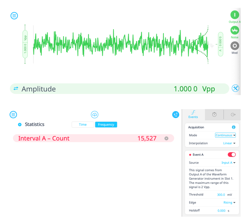
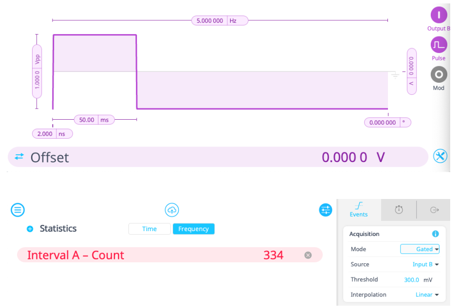
To use the Moku Time & Frequency Analyzer as an event counter, we set up the device in Multi-Instrument Mode with a Waveform Generator in Slot 1 and a Time & Frequency Analyzer in Slot 2. As seen in Figure 4, Output A of the Waveform Generator acts as the event source by generating noise. The pulse waveform on Output B will provide the gating signal.

On the Events tab of the Time & Frequency Analyzer menu, we set the source of Event A to Input A and the event threshold to 300 mV on a rising edge. We set Interval A to both start and stop upon detection of Event A. The acquisition mode will be continuous for now, so the Time & Frequency Analyzer will count a new event every time the Waveform Generator voltage rises above 300 mV. The results of this simple demonstration are shown in Figure 4, where the Interval Count statistic will keep rising until it is manually stopped or reset.

random noise — Figure 4: Configuration of the Moku Time & Frequency Analyzer for a continuous measurement of random events. Events generated by Output A continue counting for as long as the user runs the measurement.

However, it is likely in these types of experiments that we will want to measure event counts only within a certain time interval. The Moku Time & Frequency Analyzer has two settings to accommodate such requirements. The mode can be changed from continuous to windowed or gated.

Windowed mode means that the Time & Frequency Analyzer will only collect data within a limited time frame (window), and will refresh upon completion of each window. Gated mode works in a similar manner, but instead of the window refreshing automatically, it is controlled by an applied voltage signal (gate). In this demonstration, the second channel of the Waveform Generator can produce this gating signal, so we set the source to Input B and the threshold to be somewhere between 0 and 500 mV. The results are shown in Figure 5. We can compare the resulting event counts with those produced by continuous or windowed mode.

Time-interval histograms (photon counting)

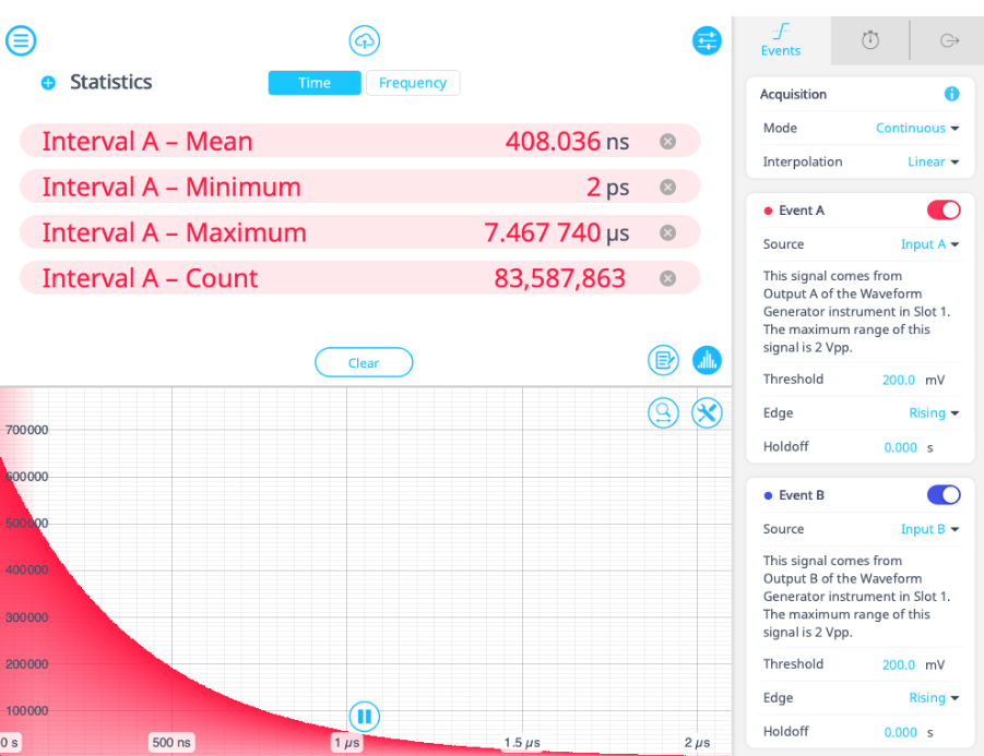
Perhaps the Time & Frequency Analyzer’s most powerful feature is its ability to accumulate measurement outcomes over time, like photon counting. In particular, time-interval histograms (see Figure 3) have become an established tool across multiple disciplines. Classic digital signal jitter measurements use the plot to aid in determining the root cause of timing errors. In essence, the histogram represents the probability distribution of the time interval error. In quantum optics, time-correlated single photon counting forms an essential part of all Hanbury-Brown-Twiss-type experiments exploring photon (anti)bunching, second- and higher-order correlation functions, two-photon quantum interference etc. [3]

To generate a time correlation between two channels, we set up the device in Multi-Instrument Mode with a Waveform Generator in Slot 1 and a Time & Frequency Analyzer in Slot 2. In this case, both Output A and Output B will provide the “events” for the Time & Frequency Analyzer instrument. Set both channels to generate noise in a manner similar to the previous example, in order to simulate random photon events.

On the Events tab of the Time & Frequency Analyzer menu, we set the source of Event A to Input A and the event threshold to 200 mV on a rising edge. Channel B will have identical settings, but with Input B as the source. Next, we set Interval A to start on Event A and stop on Event B. This measures the interval between random events on Inputs A and B. This mirrors a photon counting situation, where an event at one photodetector starts the interval and an event at the second detector stops it. We set the instrument to measure the mean, minimum, maximum, and total count of Interval A. We also enable the histogram to view the distribution of intervals, shown in Figure 6. This allows us to view the time correlation between events on A and B.

time correlation data — Figure 6: The results of the time correlation analysis between random events on two channels. The distribution centers around zero, with a mean of around 408 ns. Changing the thresholds will alter the width of the distribution.

Rise time and frequency counting

Measurement of the simple interval between two events may seem like a quotidian endeavor, but it is an extremely useful technique, enabling precision characterization in many systems. Measuring the rise- and fall-times, pulse width, and duty cycle of signals are obvious examples. Expanding our events to multiple signals opens up the possibility of phase angle measurements and a variety of sensing applications, including ultrasound, pulsed radar, and LiDAR.

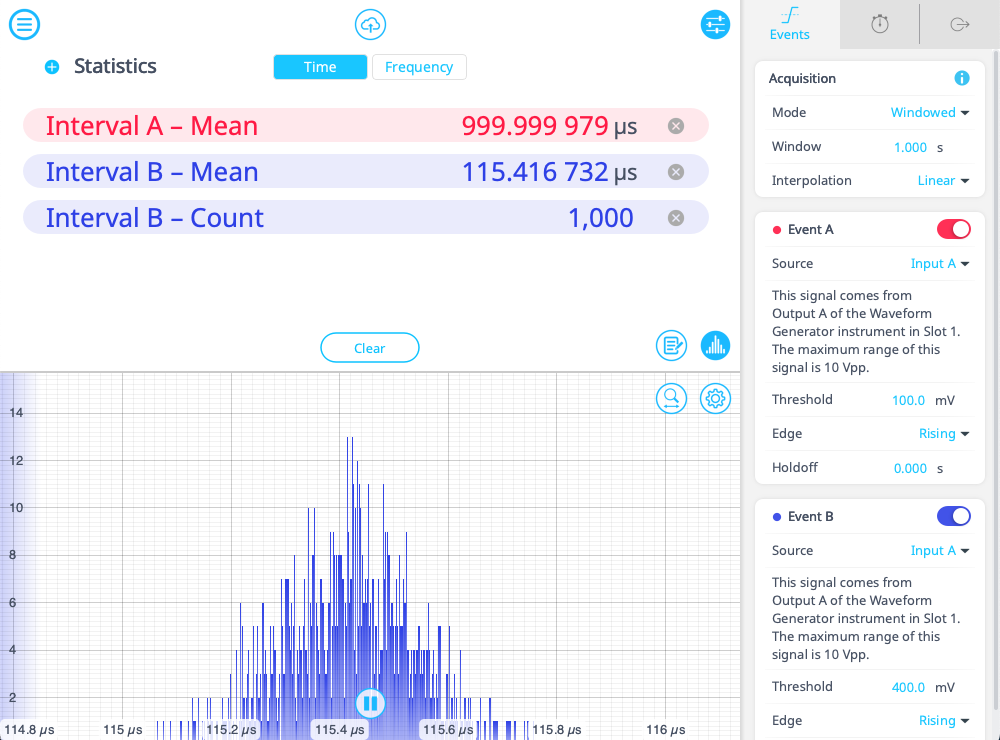
For a simple example, we can measure the frequency and rise time of a sine wave generated by the Moku Waveform Generator. First, we set up the device in Multi-Instrument Mode with a Waveform Generator in Slot 1 and a Time & Frequency Analyzer in Slot 2. Then we use the Waveform Generator to output a slow sine wave at a frequency of 1 kHz. In the Time & Frequency Analyzer, we set up two events: a rising edge at 100 mV (Event A) and another rising edge at 400 mV (Event B). On the intervals tab, we then measure two intervals, the first from Event A to Event A, which measures the period of the signal. The second, from Event A to Event B, measures the rise time of the pulse from 20% to 80% of the maximum signal. Next, we set the statistics to measure the mean of Interval A and Interval B, as well as the count of Interval B. Switching to a measurement window of 1 s, we expect 1,000 events per window, with a period of around 1 ms, as seen in Figure 7 below. Running such tests in windowed mode can give you a good idea of the frequency stability over a given period of time.

frequency counter — Figure 7: Distribution and count of events during a window of one second using the Time & Frequency Analyzer. The expected number of events in a window (1000) is detected by the instrument.

Decoding pulse-width modulation (PWM)

Pulse-width modulation (PWM) is a technique that encodes information by generating a series of pulses whose width is proportional to the amplitude of the encoded waveform. This is often used to regulate the voltage delivered to motors or LEDs, and is also used in communications. Decoding this information using the Time & Frequency Analyzer is eminently possible, as we demonstrate below.

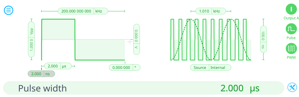
In order to decode a pulse-modulated waveform, we first set up the Moku in Multi-Instrument mode, with a Waveform Generator in Slot 1, and the Time & Frequency Analyzer in Slot 2. The Waveform generator serves as the pulse generator and is configured as seen in Figure 8. We put the Waveform Generator in pulse mode and choose a 200 kHz repetition rate with a pulse length of 2 𝛍s on Output A. We also select “PWM” mode and set the modulation rate at 1.01 kHz with a depth of ±100 ns.

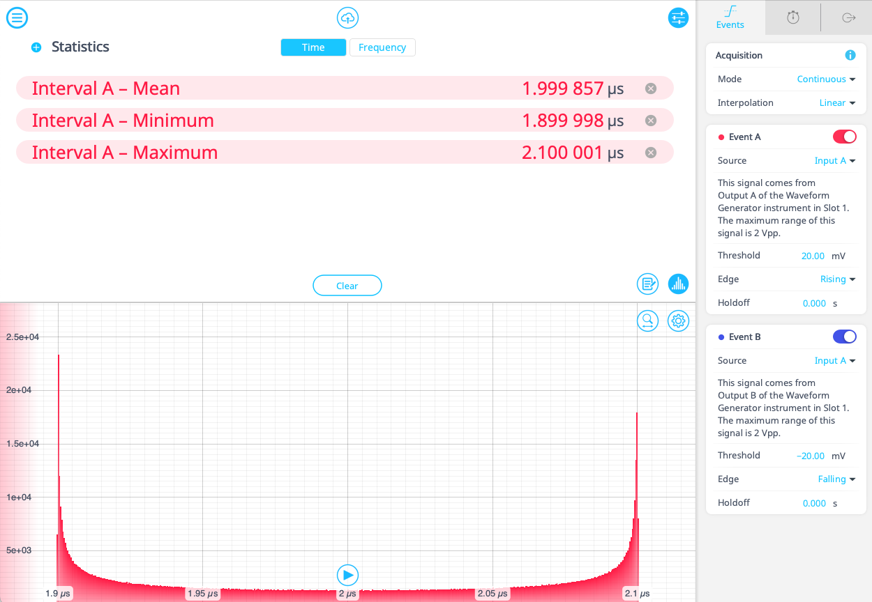
Having generated the pulse train, we now move on to the settings of the Time & Frequency Analyzer. In this case we want to track two events, both the rising and falling edge of the pulse, so that we can determine the pulse duration. We set Event A to trigger at a threshold of 20 mV on a rising edge, and Event B to trigger at -20 mV on a falling edge. Interval A tracks the time between Events A and B. We output statistics for Interval A as seen in Figure 8. Given the pulse length and modulation depth specified in the previous step, we expect a mean of 2 𝛍s, with a minimum and maximum of 1.9 𝛍s and 2.1 𝛍s respectively. We find that is indeed the result obtained by the measurement, and a histogram of the pulse length distribution is produced, allowing us to determine that the pulse modulation is working as expected.

pwm data — Figure 8: The Moku Waveform Generator creates a series of pulses with lengths centered around 2 𝛍s. The pulses are then modulated with a depth of 100 ns, creating pulses ranging from 1.9 𝛍s to 2.1 𝛍s. The Time & Frequency Analyzer is programmed to measure the width of the pulses and produces a histogram of the results. The mean, minimum and maximum calculations return the expected values.

Active Feedback

The Time & Frequency Analyzer’s analog outputs allow one to bridge the gap between time and amplitude in a way that was not previously possible.

Returning to the previous example, suppose we not only wanted to examine the results of the pulse length modulation, but view the demodulated signal on an oscilloscope trace. We would begin by returning to the Multi-Instrument Mode screen on the Moku device and adding an Oscilloscope to Slot 3, with Output A from the Time & Frequency Analyzer connected to Input A.

After reconfiguring the device, we return to the Time & Frequency Analyzer screen and view the output tab. We want the signal produced by Output A to be proportional to the interval being measured (we are not concerned with the count in this example). We set the zero point to 2 𝛍s, which is the unmodulated length of a pulse in the sequence. Since the deviation from this point is only ±100 ns, we need to set the scaling factor relatively high. We choose 10 MV/s, which will produce an oscillating wave between 1 and -1 V as the length of the pulse changes.

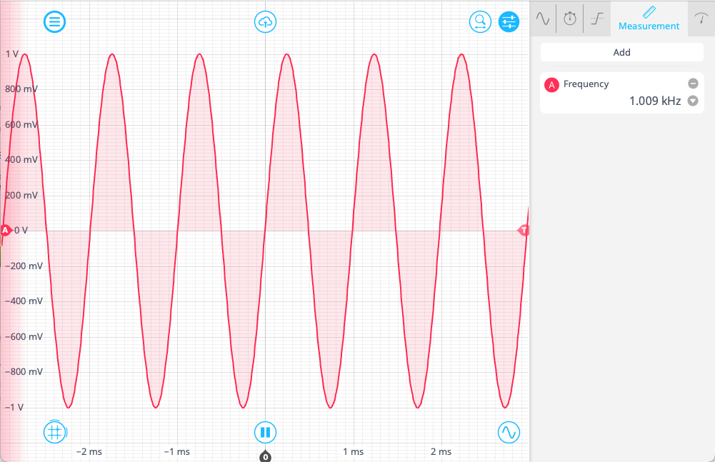
We can now view the demodulated pulse using the Oscilloscope (Figure 9). Enabling Channel A, we can see a sine wave of 1.01 kHz, which is the modulation frequency originally set in the Waveform Generator.

demodulated signal — Figure 9: A sine wave of 1.01 kHz. Originally encoded into a pulse-width modulated form by the Moku Waveform Generator, the original signal is demodulated through the Moku Time & Frequency Analyzer instrument and sent to the Oscilloscope for viewing.

Feedback loops with the Time & Frequency Analyzer

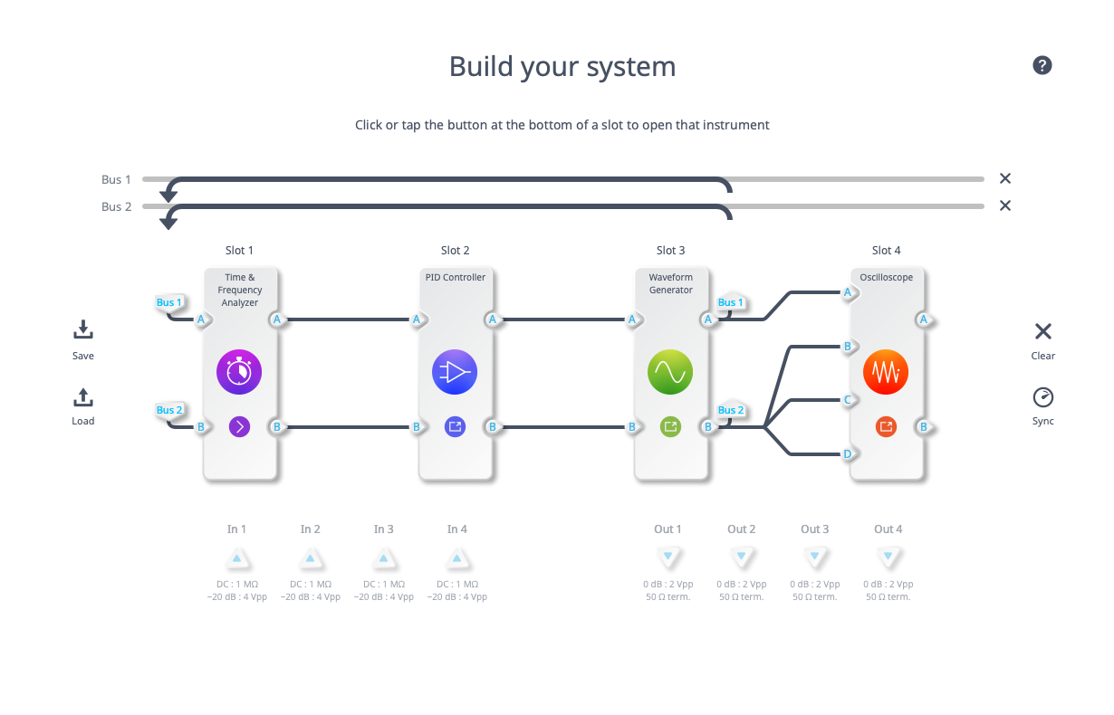
In the final example, we leverage the output voltage of the Time & Frequency Analyzer to generate a signal that follows a reference with a fixed time difference between them. The Moku configuration is seen in Figure 10, with the Time & Frequency Analyzer in Slot 1, a PID Controller in Slot 2, a Waveform Generator in Slot 3, and an Oscilloscope in Slot 4. Connect the output ports of the Waveform Generator back to the Time & Frequency Analyzer inputs via the Moku internal bus.

Figure 10: Feedback loop configuration of the Moku:Pro device.

We set up the Waveform Generator first, which provides both the reference and follower signals. Open the Waveform Generator Window and set Output B to be a standard 1 MHz sine wave. Set Output A to be a frequency-modulated sine wave with a central frequency of 1.05 MHz and a modulation depth of 100 kHz. Input A will provide the signal to be modulated. See Figure 11 for details. You can check the outputs on the Oscilloscope screen to confirm they are both enabled, although they should not be synchronized yet.

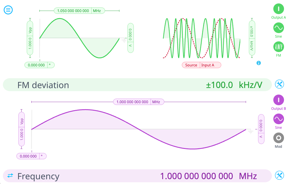
lead and follower signals — Figure 11: Settings of the Moku Waveform Generator for the feedback loop. Output A produces a frequency-modulated wave with a center frequency of 1.050 MHz, which will follow the signal on Output B. An unmodulated, 1 MHz signal is generated on Output B.

Open the Time & Frequency Analyzer and set Events A and B to trigger on a 10 mV rising edge on Inputs A and B, respectively. Interval A should be set to start on Event B and stop on Event B – essentially, the instrument will measure the time difference between the arrivals of the sine waves. On the third tab, we enable Output A and set the signal to be proportional to the interval and the zero point to be 200 ns. Change the scaling factor to 1 MV/s. The measured interval should eventually match the zero point, but first we need to set the PID controller.

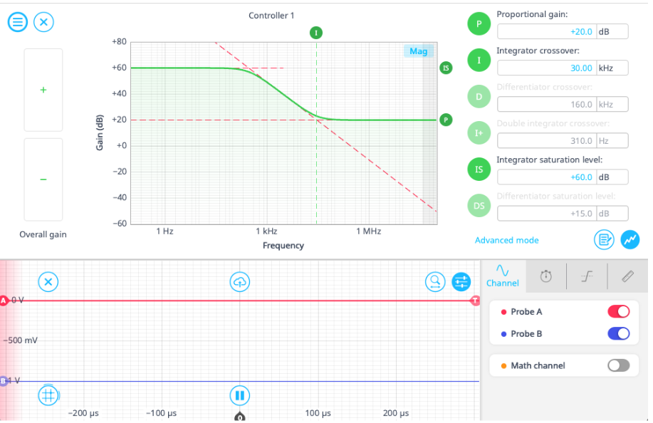
Switch to the PID controller and enable the output. Place the Probe at the input and adjust the PID parameters as necessary so that the signal turns from a periodic step to a straight line. One configuration of parameters is seen below in Figure 12, using only the proportional (P) and integral (I) terms.

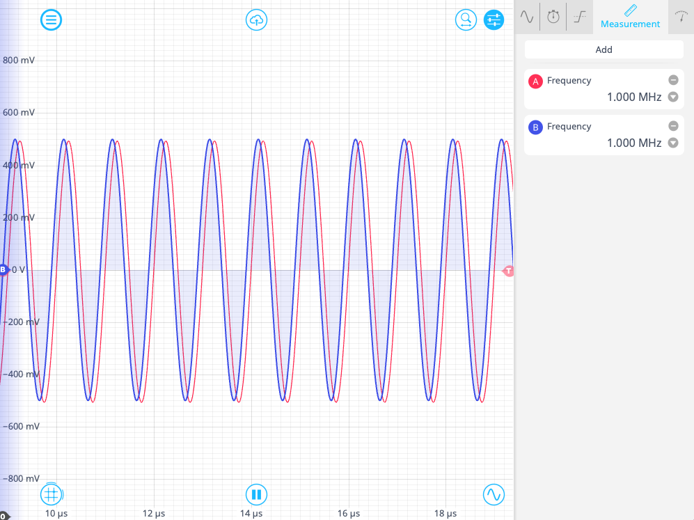
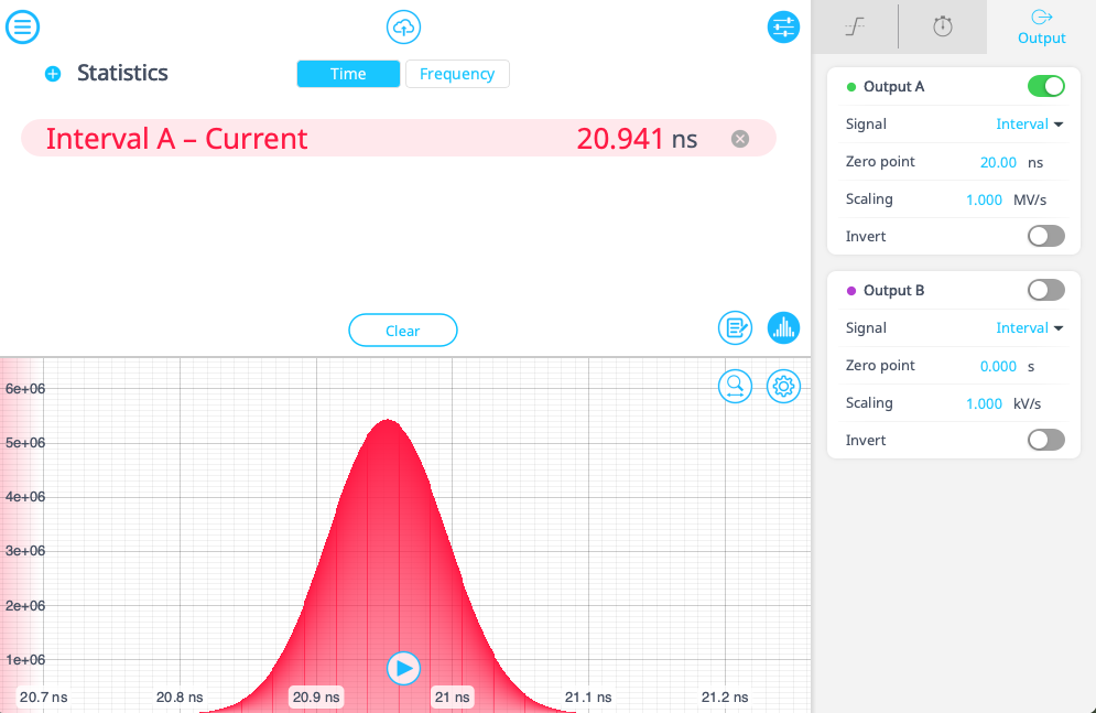
PID loop — Figure 12: The PID settings for the loop. The proportional gain should be at least 10 dB, with the integrator saturation level set to a high level (60 dB). The crossover is set to 30 kHz. The user’s exact settings may change based on the frequency and interval of interest.

Once the PID is working, switch to the Oscilloscope screen and you should see the signals time-locked on the screen, as in Figure 13. Zooming in on the signals, you should see that the offset should be approximately the same as the set point we specified for the Time & Frequency Analyzer. Finally, return to the Time & Frequency Analyzer screen and you will see a distribution of intervals centered around the set point. Try adjusting the set point and the plot will update accordingly.

Time-locked signals — Figure 13: The results of the feedback loop. Above: The time-locked signals are displayed on the Oscilloscope screen. Output A is locked to B at a frequency of 1 MHz, and the time difference between the signals is almost exactly the 20 ns that was specified in the Time & Frequency Analyzer page. Below: The interval measured by the instruments also confirms that the loop is working as intended. The preciseness of the interval relative to its stated value can be adjusted with the PID parameters.

Summary and next steps

The Time & Frequency Analyzer brings a new measurement paradigm to Moku devices, presented in an integrated environment with an intuitive interface and built-in data capture tools. A convincing standalone proposition, the Time & Frequency Analyzer also melds seamlessly with existing instruments in Multi-Instrument Mode to form bespoke testing setups and, for the most demanding applications, may be combined with custom FPGA code using Moku Cloud Compile. For additional details, check out our blog.

Learn more about the Time & Frequency Analyzer here, or explore the Time & Frequency Analyzer yourself by downloading our desktop app and selecting demo mode.

References

[1] W. E. Moerner, “Those Blinking Single Molecules,” Science, vol. 277, no. 5329, pp. 1059–1060, 1997.

[2] A. L. Efros and D. J. Nesbitt, “Origin and control of blinking in quantum dots,” Nature Nanotechnology, vol. 11, no. 8, pp. 661–671, Aug. 2016.

[3] M. Fox, Quantum optics: an introduction, ser. Oxford master series in atomic, optical, and laser physics. Oxford Univ. Press, 2006.