This application note serves as a follow-up to Part 1 of this series, Improving SNR measurement with a boxcar averager. This app note explores the configuration and operational principles of dual boxcar averagers, with an emphasis on their implementation using Moku Cloud Compile on Moku:Pro.
The working principle of dual boxcar averagers
Dual boxcar averagers are essential tools for advanced measurement techniques, particularly in pump-probe experiments and other applications sensitive to DC offsets. Expanding on the capabilities of single boxcar averagers, dual boxcar systems enhance performance by incorporating multiple synchronized single boxcar averagers.
In a pump-probe spectroscopy experiment, the pump pulse excites the sample, promoting electrons from the ground state to a vibrational or electronically excited state. The resulting intensity modulation of the probe pulse encodes critical information about molecular vibrations, population dynamics, and excited-state lifetimes. When the repetition rate of the pump laser is half that of the probe laser, only every alternate probe pulse undergoes the pump-induced modulation, while the others serve as a reference. Consequently, to accurately extract the net pump-probe signal, the system must independently integrate and analyze two consecutive probe pulses within each pump trigger period. This approach necessitates the use of two boxcar averagers to enable simultaneous signal processing of both probe pulses within each cycle.
The operational diagram for dual boxcar averagers is shown in Figure 1, where the baseline gate window and the boxcar gate window are illustrated. Both windows are activated by the same trigger signal and have the same gate width, but they are set with different trigger delays. As a result, the gate windows are shifted to align with specific parts of the input signal. In a pump-probe experiment, this setup enables the system to measure two pulses separately and calculate their difference.
The output of the dual boxcar averager is a single value representing the difference between the integrals of two pulses. This difference reflects the characteristics of the measured sample.
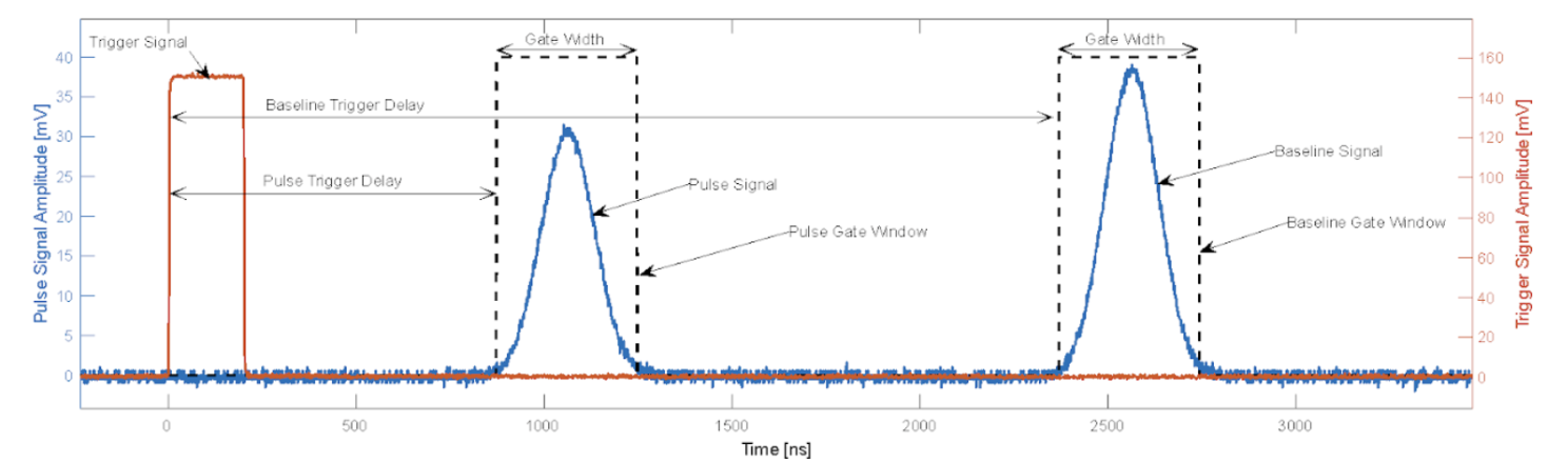
Figure 1: The operational principle of dual boxcar averagers. One pair of pulses are analyzed at the same time. The trigger signal enables two integrating boxcar gates with identical gate widths and unique trigger delays.
The implementation of dual boxcar averagers requires simply replicating the design of a single boxcar averager, with only a few additional modifications. For additional background, the boxcar averager is described in this application note. The fundamental structure of the dual boxcar averager is depicted in Figure 2. The “Single Boxcar” denotes a fully functional single boxcar averager with dedicated control registers. The changes include introducing extra subtractors and a signal selection mechanism to manage multiple signals at the output stage.
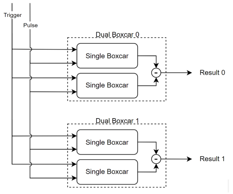
Figure 2: A block diagram of a dual boxcar averager. Each “Single Boxcar” is a fully functional boxcar averager block that receives one pulse signal and one trigger signal to perform one boxcar averager. The dual boxcar averager includes two sets of boxcar averagers. Two results of the boxcar averagers will be subtracted to extract the differential measurement.
The constructed boxcar averager has two pairs of dual boxcar averagers instead of one. Some applications go further, requiring not only the differential measurement between two pulses, but also the absolute intensity of each pulse with the baseline subtracted. To address this need, a second set of dual boxcar averagers is introduced, with one boxcar integrating the pulse signal and the other one integrating the DC baseline. By removing the baseline, the system recovers the absolute intensity of laser pulse signals and minimizes background noise. This approach is particularly important as fluctuations in the baseline can introduce unwanted noise, reducing the precision and reliability of the measurements.
This application note focuses on operational guidance. For more details about the structure, refer to the Simulink model on GitHub.
Implementing dual boxcar averagers
The operation of dual boxcar averagers follows the same fundamental process as a single boxcar averager. However, dual boxcar averagers offer multiple output modes, allowing users to select and output values computed by different averagers.
This section outlines how to operate dual boxcar averagers on Moku:Pro using a Python control panel and Moku Cloud Compile control registers. The Python control panel, developed with the Moku Python API, provides a graphical interface for controlling the dual boxcar averagers. A key advantage of this interface is its ability to automatically convert between bits, volts, and nanoseconds, simplifying the configuration process. In contrast, while the Moku Cloud Compile control registers also offer full control, they require manual value conversions, a topic explored in more detail later in this application note.
Python control panel
(1) Adjusting the trigger level
In this experiment, the trigger signal has an amplitude of 150 mV. Setting the trigger level to 75 mV ensures reliable and stable triggering for boxcar integration. The boxcar window appears only when the system is properly triggered; otherwise, neither the stable pulse signal nor the trigger signal will be visible. Figure 3(a) illustrates a scenario where the boxcar window fails to activate because the trigger level is set higher than the trigger signal amplitude.
Figure 3(b) displays two boxcar windows with intentionally different amplitudes to distinguish between the pulse boxcar and the baseline boxcar. The larger amplitude corresponds to the pulse boxcar, while the smaller amplitude represents the baseline boxcar.
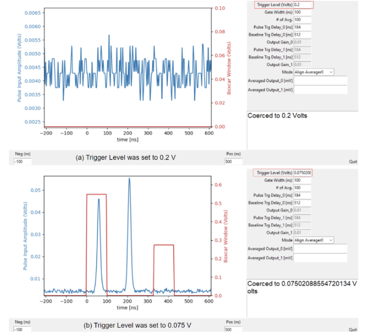
Figure 3: System responses under different trigger level settings. (a) When the trigger level is set to 0.2 V, which exceeds the trigger signal amplitude of 0.15 V, the boxcar window fails to activate. As a result, neither the boxcar window nor the pulse signal is present. (b) Lowering the trigger level to 0.075 V — half the amplitude of the trigger signal — successfully triggers both boxcar windows, as shown by the red traces in the graph. The pulse boxcar gate exhibits a larger amplitude, whereas the baseline boxcar gate has a smaller amplitude.
(2) Aligning the triggered boxcar gate windows with the pulse signal and configuring the gate width
In this step, the trigger delay and boxcar gate width are optimized to precisely match the characteristics of the input signals. Since the system includes two pairs of dual boxcar averagers, the first task is to select which averager to configure. Setting the mode to “Align Averager0” allows adjustment of the trigger delay for the first dual boxcar averager.
The trigger delays are set to ensure the boxcar windows align with the start of the pulses of interest. Once aligned, the gate width is adjusted to integrate most of the pulse duration, as shown in Figure 4. Both boxcar windows are configured to use the same gate width for consistency.
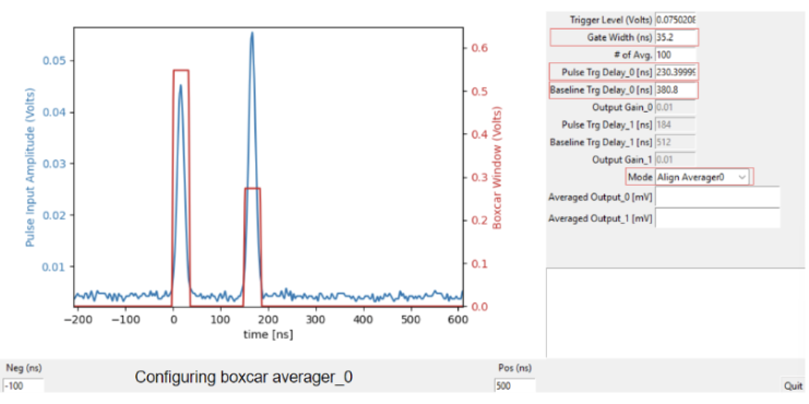
Figure 4: The configuration of Averager0. The configuration mode is set to “Align Averager0” to adjust the first dual boxcar averager. The gate width is set to 35.2 ns, with a pulse trigger delay of 230.4 ns and a baseline trigger delay of 380.8 ns. These two boxcar windows are properly aligned with the pulses, ensuring accurate signal integration.
Next, the trigger delays and gate width for Averager1 can be adjusted if an extra dual boxcar averager is needed. Like the previous step, two integrator gates are configured to analyze the corresponding signals. In Figure 5, the setup analyzes both the pulse and baseline signals. Consequently, the output from Averager1 represents the absolute signal amplitude of the first pulse.
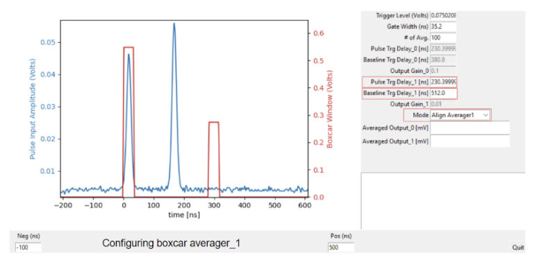
Figure 5: The configuration of Averager1. The output mode is set to “Align Averager1.” The pulse trigger delay is set to 230.4 ns, identical to Averager0. However, the baseline trigger delay is set to 512 ns to measure the DC offset. This baseline trigger delay can be adjusted if the baseline boxcar window is configured to capture only the DC offset.
For proper operation, the trigger delay difference must be greater than the pulse width. In Figure 6, the trigger delay difference is 25.6 ns, which is less than the gate width of 35.2 ns. As a result, the two boxcar gates overlap, leading to unintended behavior and triggering a warning message in the user interface.
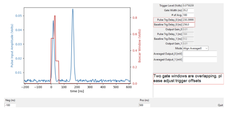
Figure 6: An incorrect setup of trigger delays and gate width. The trigger delay difference is 25.6 ns, determined by subtracting the pulse trigger delay of 230.4 ns from the baseline trigger delay of 256 ns. Since the resulting value is smaller than the gate width, there is an overlap between the boxcar gates. Consequently, the displayed boxcar windows (red trace) show a large abnormal peak, indicating the overlap of gates.
(3) Selecting number of averaging periods and adjusting the gain stage
Each averager outputs the difference between the pulse integrator and the baseline integrator. Proper configuration of the output gain is essential, as incorrect settings can cause output saturation. If saturation occurs, a warning message will appear in the text box (Figure 7). To correct this, the output gain should be reduced.
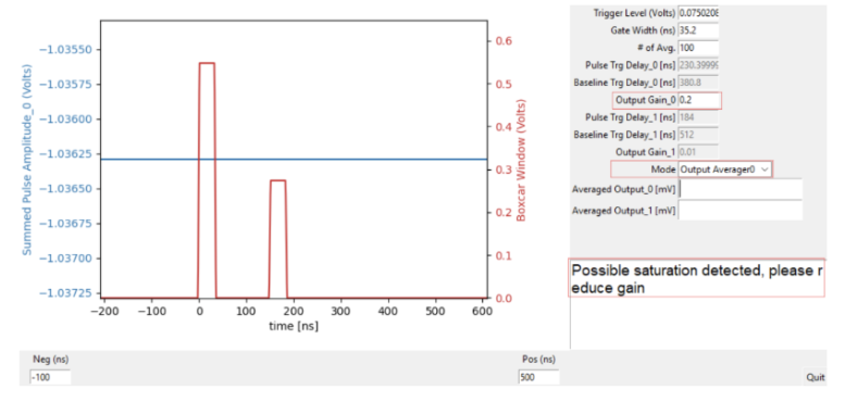
Figure 7: Output saturation caused by a high output gain. The mode is set to “Output Averager0” to display results from Averager0. The gain is configured to 0.2, resulting in an output of approximately -1.036 V, which is close to the -1.095 V saturation limit of Moku:Pro. A saturation warning is generated, indicating that the output gain is too high.
The output of the boxcar averager is the sum of n boxcar integrated results rather than the average. This design choice is due to the computational complexity and resource demands of implementing a divider on an FPGA. Outputting the integrated results directly is more efficient than computing the actual average. When the output gain is properly configured, as shown in Figure 8, the averager output is displayed on the interface. The “Averaged Output_0” represents the rescaled real value, which is obtained by dividing the raw integration output by both the number of averages and the output gain. For instance, the raw value obtained from the boxcar averager output is approximately -0.5556 V, as shown on the scope. However, the displayed “Averaged Output_0” value is around -55.56 mV. This reduction by a factor of 10 is due to the averaging factor of 100 and a gain setting of 0.1, resulting in an overall raw gain of 10 for the averager in this case.
\(\text{Averaged} = \frac{\text{Summed Pulse Amplitude}}{\text{# of Avg.} \times \text{Gain}}\)
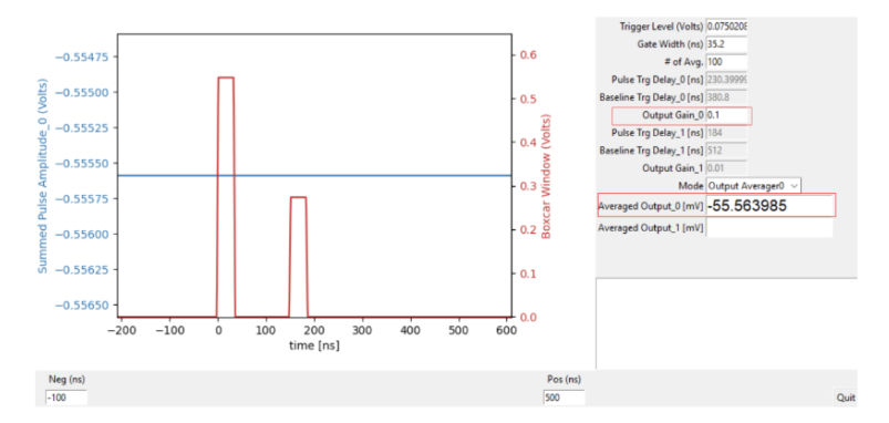
Figure 8: Rescaled averager output with a proper output gain. The output gain is set to 0.1, and the averaged value is displayed as -55.56 mV. However, the scope reading (blue trace) shows approximately -0.5556 V. This discrepancy arises because the displayed value is rescaled to be 10 times smaller, resulting from the combined effect of a raw gain of 10 — determined by the 100 averaging factor and the 0.1 gain setting.
Additionally, results from both averagers can be displayed simultaneously. By setting the output Mode to “Output Both,” users can view both outputs. The blue line in Figure 9 represents the results from Averager0, while the red line corresponds to Averager1. The data is streamed directly from Moku:Pro, and it can be further processed and analyzed using the Moku API.
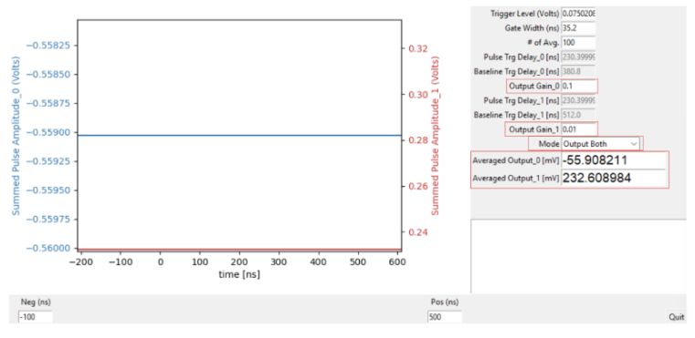
Figure 9: Simultaneous output display of both averagers. The output mode is set to “Output Both” to enable the outputs of both dual boxcar averagers. The output gain is configured to 0.1 for Averager0 and 0.01 for Averager1. The averaged output values are then displayed on the control panel as -55.9 mV and 232.6 mV, respectively.
Moku Cloud Compile control registers
The dual boxcar averagers can also be controlled by manually adjusting the Moku Cloud Compile control registers within the Moku app. Table 1 outlines the functions associated with each port. The table is organized into three sections: the I/O port definitions and shared control registers, followed by two separate sets of control registers: one for Averager0 and the other for Averager1. This structure allows for complete control over both boxcar averagers.
Table 1: Configurations of boxcar averager input, control, and output ports.
| Signal ports | Data types | Explanations |
|
Shared I/O ports and control registers |
||
| InputA | Signed 16-bit | Input pulse signal |
| InputB | Signed 16-bit | Trigger signal |
| OutputA | Signed 16-bit | Boxcar averager output signal (single & dual-output modes)
Input pulse signal (align mode) |
| OutputB | Signed 16-bit | Boxcar gate window (align mode & single-output mode)
Boxcar averager output signal (dual-output mode) |
| Control0 | Signed 16-bit | Trigger level, active on the rising edge |
| Control15 | 4-bit | Control15 = 4 : Output both box averagers
Control15 = 7 : Output averager_0 Control15 = 9 : Output averager_1 Control15 = 13: Align averager_1 Control15 = 15: Align averager_0 |
|
Boxcar averager_0 control registers |
||
| Control1 | Unsigned 16-bit | PulseTriggerDelay_0, in the unit of clock cycle |
| Control2 | Unsigned 16-bit | BaselineTriggerDelay_0, in the unit of clock cycle |
| Control3 | Unsigned 16-bit | GateWidth_0, in the unit of clock cycle |
| Control4 | Unsigned 16-bit | AvgLength_0, Averager length, in the unit of results from boxcar integrator |
| Control5 | Unsigned 32-bit | Gain_0, Output signal gain, for re-scaling results to 16-bit signals.
The lower 16 bits of Control5 are configured as fractional gain. |
|
Boxcar averager_1 control registers |
||
| Control6 | Unsigned 16-bit | PulseTriggerDelay_1, in the unit of clock cycle |
| Control7 | Unsigned 16-bit | BaselineTriggerDelay_1, in the unit of clock cycle |
| Control8 | Unsigned 16-bit | GateWidth_1, in the unit of clock cycle |
| Control9 | Unsigned 16-bit | AvgLength_1, Averager length, in the unit of results from boxcar integrator |
| Control10 | Unsigned 32-bit | Gain_1, Output signal gain, for re-scaling results to 16-bit signals.
The lower 16 bits of Control10 are configured as fractional gain. |
(1) Adjusting the trigger level
The Moku Cloud Compile block control registers are configured with the values shown in Figure 10 (b). The Switch Control is set as 15 to configure Averager0. The Trigger Level is set to 2,244, corresponding to a trigger threshold amplitude of \(75 \text{mV}\) ( \(\frac{\text{2244 LSBs}}{\text{29925 LSBs/V}} \approx 75 \text{mV}\) where LSB stands for least significant bit and \(29925 \text{ LSBs/V}\) is the digital resolution of Moku:Pro). It is obvious that no boxcar window is triggered in Figure 10(a) because the Trigger Level is set to 0.2 V \(\left( \frac{5985 \text{ LSBs}}{29925 \text{ LSBs/V}} \approx 200 \text{ mV} \right)\), which is higher than the trigger signal amplitude.
Prior to the alignment process, the Trigger Delay can be set to 0. For a Gate Width of 320 ns, its control register is configured as \(\frac{320 \text{ ns}}{T_{clk}} = 100\), where \(T_{clk} = \frac{1 \text{ s}}{312.5 \text{ MHz}} = 3.2 \text{ ns}\) on Moku:Pro.
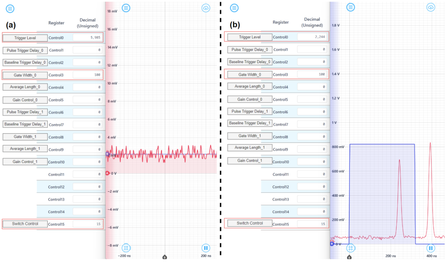
Figure 10: Initial configuration of the Moku Cloud Compile control registers. (a) The trigger level is set to 0.2 V, and no boxcar windows are triggered. (b) The trigger level is set to 75 mV, and the gate width is configured to 320 ns, resulting in the display of a 320 ns boxcar window (blue trace).
(2) Aligning the triggered boxcar gate windows with the pulse signal and configuring the gate width
Here, the adjustment begins by setting the Gate Width to \(11 \times 3.2 \text{ns} = 35.2 \text{ns} to match the pulse width. Next, the Pulse Trigger Delay is set to \)latex 72 \times 3.2 \text{ns} = 230.4 \text{ns}$, followed by the configuration of the Baseline Trigger Delay to \(119 \times 3.2 \text{ns} = 380.8 \text{ns}\). As shown in Figure 11, this adjustment successfully aligns the blue (boxcar windows) and red (pulses) traces, ensuring that each pulse is properly integrated with its corresponding boxcar window.
Figure 11 illustrates two boxcar windows, each with a distinct amplitude to differentiate the pulse boxcar from the baseline boxcar. The larger amplitude corresponds to the pulse boxcar, while the smaller amplitude represents the baseline boxcar. Both boxcar windows are configured to use the same gate width for consistency.
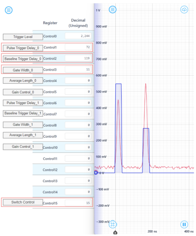
Figure 11: Configuration of trigger delays and gate width for boxcar integration. The gate width is set to 35.2 ns, with a pulse trigger delay of 230.4 ns and a baseline trigger delay of 380.8 ns. The taller gate window is the pulse boxcar gate, and the shorter one is the baseline boxcar gate, ensuring proper integration of the target pulses.
After configuring Averager0, the Trigger Delays and Gate Width for Averager1 can be adjusted if an extra dual boxcar averager is needed. Like the previous step, two integrator gates are set up to analyze the corresponding signals. In Figure 12, the configuration captures the probe pulse and the baseline (DC level) signal. As a result, the output from Averager1 reflects the absolute signal amplitude of the first pulse.
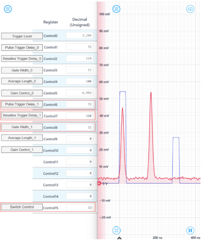
Figure 12: Configuration of Averager1. The switch control was configured as 13 to visualize the boxcar windows of Averager1. The baseline trigger delay was configured to 160×3.2 ns=512 ns, positioning the baseline boxcar in an empty region where it only integrates the DC offset.
For proper operation, the trigger delay difference must be greater than the pulse width. In Figure 13, the trigger delay difference is $latex (79-72) \times 3.2 \text{ns} = 22.4 \text{ns}, which is less than the gate width of 35.2 ns. This causes the two boxcar gates to overlap, which is not intended, and an abnormal peak can be observed in the blue line.
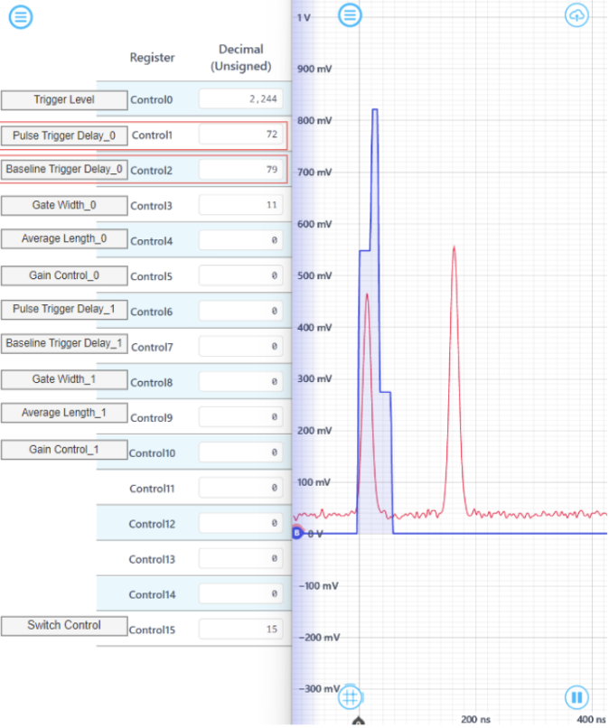
Figure 13: Incorrect setup of trigger delays and gate width. The trigger delay difference is 22.4 ns, which is smaller than the gate width, leading to an overlap between the boxcar gates. Consequently, the boxcar windows displayed (blue trace) show a large abnormal peak, indicating the overlap of gates.
(3) Selecting the number of averaging periods and adjusting the gain stage
Each averager generates an output representing the difference between the pulse integrator and the baseline integrator. Proper configuration of the output gain is crucial, as incorrect settings can result in output saturation. If saturation occurs, the output gain should be reduced accordingly.
The Gain Control is set to 65,536 in Figure 14(b), effectively configuring the least significant 16 bits (fractional bits) as all zero and the integer gain (the most significant 16 bits) as one. This establishes a unity gain for the boxcar averager output. If noticeable quantization errors occur, this value can be increased to amplify the output. For example, setting this control register to 655,360 applies a 10x gain, whereas lowering it to 32,768 results in a 0.5x attenuation to prevent saturation.
In Figure 14(a), the gain control is set to 6,553, corresponding to a 0.1x attenuation. As a result, the output is –557.26 mV, which falls within the acceptable output range. In Figure 14(b), the readout value is –1.0950 V, which represents the saturation limit of Moku:Pro, indicating that Averager0 is saturated under this configuration. To avoid saturation, the gain should be reduced.
As discussed, the output of the boxcar averager is the summation of the integrated results from n boxcar windows, rather than the average. This approach is preferred because implementing a divider on the FPGA is resource-intensive and time-consuming. Therefore, outputting the integrated results is more efficient than computing the actual average. And the recovered value is \(\frac{-557.26 \text{ mV}}{100 \times 0.1} = -55.726 \text{ mV}\).
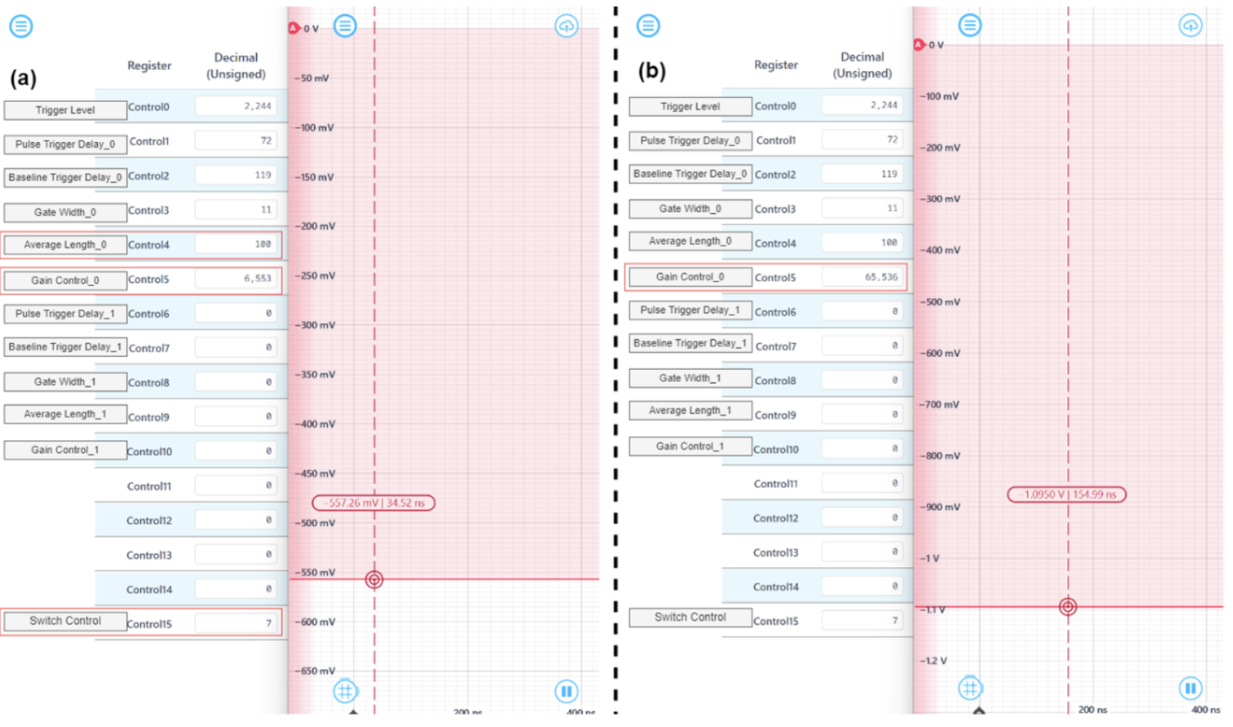
Figure 14: Averager0 output with different gain settings. (a) The switch control is set to 7 to display results from Averager0. The average length is configured to 100, averaging 100 points from the boxcar integrator, with the gain set to 6,553 to apply a 0.1x attenuation. (b) The gain factor is increased to 65,536, resulting in a unity gain. This causes saturation, as indicated by the output value of –1.0950 V, which is the minimum output value of Moku:Pro.
Additionally, the dual boxcar averagers are capable of outputting results from both boxcar averagers simultaneously. Two channels are used to display these values: the red channel (InA) represents the Averager0 output, while the blue channel (InB) corresponds to the Averager1 output. These outputs can be acquired using either the Moku Data Logger or the Moku API for further data processing and analysis.
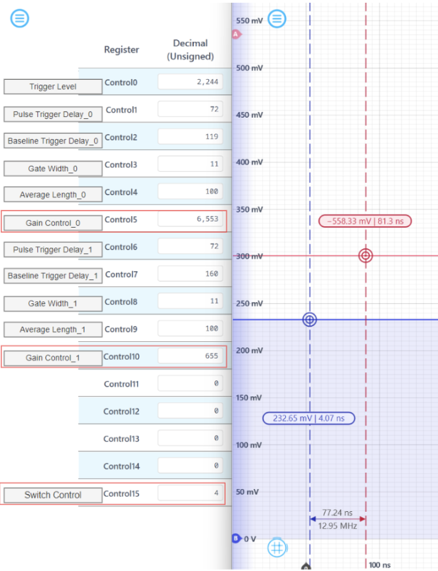
Figure 15: The dual boxcar averager outputs. The switch control is set to 4 to output the results from both averagers. The gain is configured to 0.1 for Averager0 and 0.01 for Averager1 to prevent saturation. Under these settings, the measured output values are –558.33 mV for Averager0 and 232.65 mV for Averager1.
Summary
This application note examines the implementation of a dual boxcar averager, outlining its core structure, which comprises four single boxcar averagers grouped into two pairs. Each pair generates a differential output by calculating the difference between the pulse and baseline integrators. The note also explores configuration options, including a Python control panel and Moku Cloud Compile control registers, for seamless operation. This enhanced design makes the dual boxcar averager particularly well-suited for pump-probe experiments, offering an efficient solution for automated multi-boxcar processing and differential result generation.