

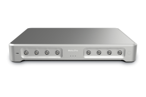

Moku Version 3.3 brings a new Neural Network instrument to Moku:Pro that enables users to implement artificial neural networks for fast, flexible signal analysis, denoising, sensor conditioning, closed-loop feedback, and more. If you are unfamiliar with the basics of a neural network or want to know how one can benefit your research and development goals, read on to explore real-life applications and tutorials.First, it’s important to note that “artificial neural network” (ANN) is the more accurate term for these systems, since they are software-based, rather than biological neurons. With this clarification in mind, we will use the term “neural network” to refer to an ANN. For this introduction, we’ll consider only fully connected neural networks, rather than complicated setups such as convolutional, recurrent, and transformer architectures.A neural network is a system of interconnected nodes, or neurons, arranged in layers. The first layer takes external data as its input. Each subsequent neuron computes a weighted sum of its inputs from the previous layer, and then adding a value called a bias. This value is then passed through an activation function, which introduces non-linearity, enabling the network to learn complex patterns. The final layer produces the network’s output, while all layers in between are known as hidden layers. Through training, the network adjusts its weights and biases to improve its accuracy over time.In mathematical terms, imagine the input layer as an N ✕ 1 matrix, where N is the number of nodes in the input layer and each element in the matrix corresponds to the activation value, as shown in Figure 1.
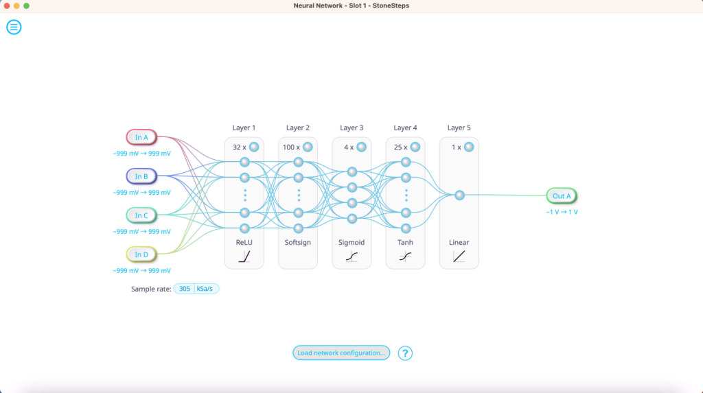
Figure 1: Neural network architecture, showing input, hidden, and output layers.Next are the hidden layers. The number of hidden layers and nodes within them depends on the complexity of the model and available computational power. The activations in the hidden layers are calculated using a combination of the activations from the previous layer, with each node applying different weights and biases to the input layer values. This is shown in linear algebra terms in Figure 2.
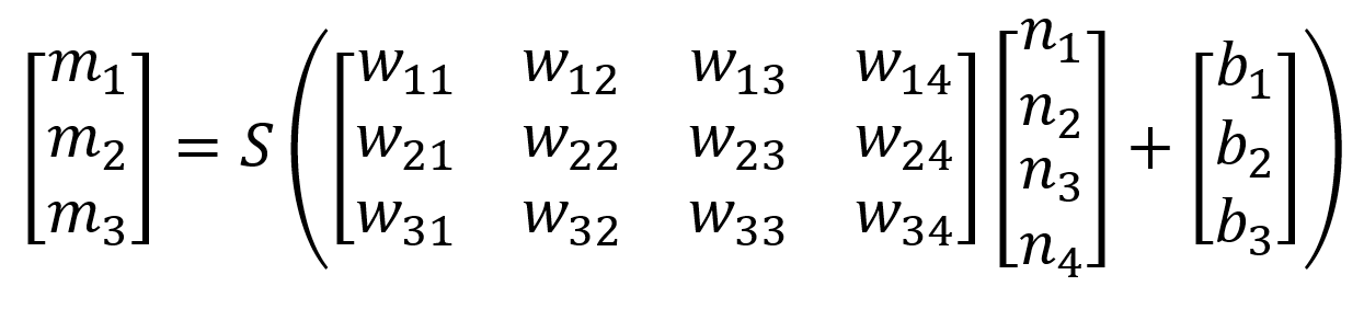
Figure 2: The activations in the hidden layers are calculated using a combination of the activations from the previous layer.If the input layer is an N ✕ 1 matrix (\(n_1\), \(n_2\)), the next activations are obtained by multiplying this with an M ✕ N matrix, where M is the number of nodes in the hidden layer. Each element in the matrix is a weight represented by \(w_{mn}\), meaning that MN parameters are needed for each layer. The result is an M ✕ 1 matrix, which is then offset by a bias value (\(b_1\), \(b_2\)…). After calculating the new activations, they are passed through an “activation function”. The activation function can provide nonlinear behavior such as clipping and normalizing, making the network much more powerful than it would be if it were simply a series of matrix multiplications. Each activation function has distinct properties, and the “correct” choice depends heavily on the application. Common options include ReLU (Rectified Linear Unit), which is computationally efficient but can struggle with certain training scenarios, as it truncates negative values. Others, like Tanh and Sigmoid functions, produce smooth, bounded outputs useful for classification but can weaken learning in deep networks, with the curve flattening out at large input values. Lastly, Linear functions work well for regression tasks but limit the network’s ability to model complex, non-linear patterns. Different layers can use different activation functions, and the choice depends on the specific application requirements and network architecture. After passing through several hidden layers, the data finally arrives at the output layer. In the output nodes, the value of the activation corresponds to some parameter of interest. As an example, suppose that time series data collected from an oscilloscope is fed into the input, and the goal of the network is to classify the signal as a sine wave, square wave, sawtooth wave, or DC signal. In the output layer, each node would correspond to one of these options, with the highest value activation representing the network’s best guess as to the form of the signal. If one activation is close to 1 and the others are close to 0, the confidence of the network’s guess is high. If the activations are similarly valued, this indicates low confidence in the answer.
How do neural networks work?
Without adjusting the weights and biases of the hidden layers, a neural network ends up being nothing more than a complex random number generator. To improve the accuracy of the model, the user must provide training data, where both the input dataset and expected answer are known. The model can then calculate its own answer to the training set, which can be compared to the true value. The calculated difference, known as the cost function, gives a quantitative assessment of the model’s performance. The model aims to reduce this cost function through training. For instance, Mean Squared Error (MSE) finds the average of the squared differences between the predicted and real values. An optimizer is the method used to efficiently minimize this cost function. Machine learning packages for Python, such as Keras, help guide the choice of the right cost function and optimizer. After calculating the cost function for a given dataset, the weights and biases of the hidden layers can then be adjusted through various calculus operations, with the goal of minimizing the cost function. This is similar to the concept of gradient descent in vector calculus and can be explored further in literature [1]. This process, called backpropagation, allows information obtained via the cost function to work backward through the layers, resulting in the model learning, or adjusting itself, without human input.Training data is often run through the neural network multiple times. Each instance of this data being provided to the model is known as an epoch. Typically, some training data will be reserved for validation. In validation, a trained network is used to infer outputs from this reserved data set and its predictions compared to the known correct output. This gives a more accurate picture of the model’s performance than the cost function value alone, as it indicates how well the model can generalize results to new and novel inputs.
What are the different types of neural networks?
Neural networks, while operating on similar principles, can take various forms depending on the application. A few common neural network examples include:
- Feed-forward neural network (FNN): This is the standard format, such as the one discussed in the above examples. In an FNN, data is passed forward through the network without any feedback or memory of the previous input. A typical example is an image, where each pixel is an input into the neural network, and the output is a classification of that image.
- Convolutional neural network (CNN): This is a subtype of FNN that is commonly used to detect features in images through the use of filters. Given the typically large size of images, these filters act to reduce the dimensions of the input image into a much smaller number of weights. Each neuron in the hidden layer can then scan for the same feature over the entire input, making CNNs robust to translation of images.
- Recurrent neural network (RNN): As opposed to feed-forward networks, RNNs involve the use of feedback in the hidden layers. Feedback mechanisms give the system a memory, so that the output of a given layer can depend on prior inputs. This makes RNNs excellent choices for sequential data sets such as time series, speech, and audio data.
- Autoencoder: An autoencoder is a special configuration of a neural network, typically an FNN or CNN, that encodes a given data into a reduced dimensional space, and then reconstructs, or decodes, it from the encoded data. Conceptually, this is very similar to principal component analysis (PCA), which is useful in statistics and bioinformatics.
How are neural networks used in signal processing?
While neural networks are popular for things like powering large language models, deciphering images, and translation, they are also incredibly useful for signal processing. A few examples where machine learning can improve a measurement setup include:
- Control systems: In some systems, the inputs required to achieve a particular control state are hard to know in advance, or put differently, the plant model is hard to invert. In such cases, a waveform generator or function generator probes the plant, while an oscilloscope monitors the resulting state. The neural network then learns the reverse mapping from the difference between the current state and the required control. When used in conjunction with a PID controller, this could enable the self-tuning of PID parameters [2].
- Sensor conditioning: A neural network can take sensor data and compensate for systematic errors, such as phase distortion or delay in cables, or beam misalignment in a photodetector. This approach allows data to be corrected before it is passed to the next stage of the experiment.
- Signal denoising: This technique uses the neural network as an autoencoder to pull out the key features of a signal, and then reconstructs it based on these features. Random noise is not a key feature, so the reconstructed signal should be noise-free, essentially using the neural network as a noise filter, as seen in Figure 3.
- Signal classification: The neural network can compare an input signal, such as a time series, to a known template or series of templates. This enables the user to quickly categorize signal classes, identify outliers or errors in a dataset, detect random events, or identify quantum states based on IQ quadrature amplitudes [3].
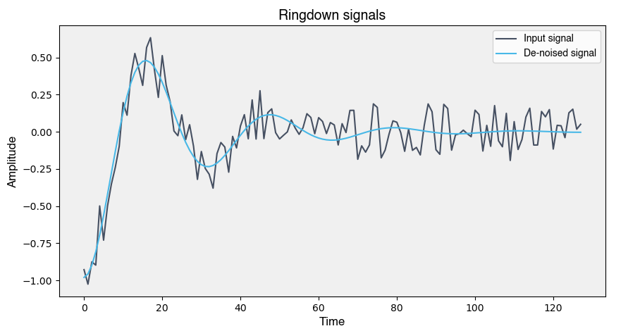
Figure 3: A reconstructed, denoised signal after being fed through a neural network.
What are the benefits of an FPGA-based neural network?
Neural networks are typically built and run on combinations of CPUs and/or GPUs. This approach gives incredible computing power, but it is also resource intensive. Large AI models are energy hungry and often excessive for the types of signal processing applications previously mentioned.FPGAs, by comparison, are not as intrinsically powerful as high-end computers. However, their flexibility makes them strong candidates for implementing small-scale neural networks. Their parallel processing capability benefits the linear algebra and other complex mathematics involved in the forward and backward propagation of information through the network. Larger neural networks often require an increased number of cycles for feed-forward passes on an FPGA because single-cycle processing is constrained by the FPGA’s spatial capacity and associated memory.FPGA-based neural networks are ideal for experimental situations, as their speed in handling real-time data enables rapid control and decision-making, without having to communicate with a host PC. FPGAs are also reconfigurable, so the user can quickly configure the neural network to their own needs. Lastly, given their compact size, neural networks implemented on FPGAs can help reduce resource and energy consumption [4][5].
What is the Moku Neural Network?
In addition to a reconfigurable suite of fast, flexible, FPGA-based test and measurement instruments, Moku:Pro now offers the Moku Neural Network. Benefiting from the versatility and fast processing speed of FPGAs, the Neural Network can be used alongside other Moku instruments such as the Waveform Generator, PID Controller, and Oscilloscope in applications such as signal analysis, denoising, sensor conditioning, and closed-loop feedback. You can use Python to develop and train your own neural networks and upload them to Moku:Pro using the Moku Neural Network in Multi-Instrument Mode. This allows for analysis of up to four input channels, or one channel of time series data, and up to four outputs for processing experimental data in real time — all on Moku:Pro. The Moku Neural Network features up to five dense layers of up to 100 neurons each, and five different activation functions depending on your application. If you’re interested in seeing how the FPGA-based Moku Neural Network can benefit your research, check out this step-by-step tutorial. This guide walks through all the basics, including Python installation, Moku Neural Network construction and training, and implementation. If you’re already familiar with the fundamental concepts of a neural network, you can find advanced, ready-to-use examples here. Prefer a video tutorial? Watch our webinar on demand. You’ll learn how to implement an FPGA-based neural network for fast, flexible signal analysis, closed-loop feedback, and more.
Citations
[1] K. Clark, Class Lecture, Topic: “Computing Neural Network Gradients,” CS224n, Stanford University, USA, 2019. https://web.stanford.edu/class/cs224n/readings/gradient-notes.pdf[2] J. Wang, M. Li, W. Jiang, Y. Huang, and R. Lin, “A Design of FPGA-Based Neural Network PID Controller for Motion Control System.” Sensors, vol. 22, no. 3, p. 889, Jan. 2022. https://doi.org/10.3390/s22030889 [3] N. R. Vora et al., “ML-Powered FPGA-based Real-Time Quantum State Discrimination Enabling Mid-circuit Measurements,” arXiv:2406.18807 [quant-ph], Jun. 2024. https://arxiv.org/abs/2406.18807 [4] A. El Bouazzaoui, A. Hadjoudja, O. Mouhib, “Real-Time Adaptive Neural Network on FPGA: Enhancing Adaptability through Dynamic Classifier Selection,” arXiv:2311.09516v2 [cs.AR], Nov. 2023. https://arxiv.org/html/2311.09516v2[5] C. Wang and Z. Luo, “A Review of the Optimal Design of Neural Networks Based on FPGA,” Appl. Sci., vol. 12, no. 3, p. 10771, Oct. 2022. https://doi.org/10.3390/app122110771