In Part 1 of this white paper, we introduced 2-level quantum systems known as qubits, which are used in various applications ranging from quantum computation to magnetic field sensing. We examined a few examples of how qubits are physically implemented, as well as the structure of a generic two-level quantum system.

In this second part, we introduce the graphical representation of qubit states known as the Bloch sphere. We also use this model to demonstrate how common pulse sequences such as Rabi, Ramsey, and CPMG can be implemented on reconfigurable hardware such as Moku to extract key information from these qubits. 

Download and read the entire white paper here.

The Bloch sphere

To visualize the state and time evolution of a two-level quantum system, we introduce a helpful tool called the Bloch sphere. Originally developed to describe the behavior of a classical ensemble of nuclear spins, the Bloch sphere has since become the standard way to represent two-level quantum states.

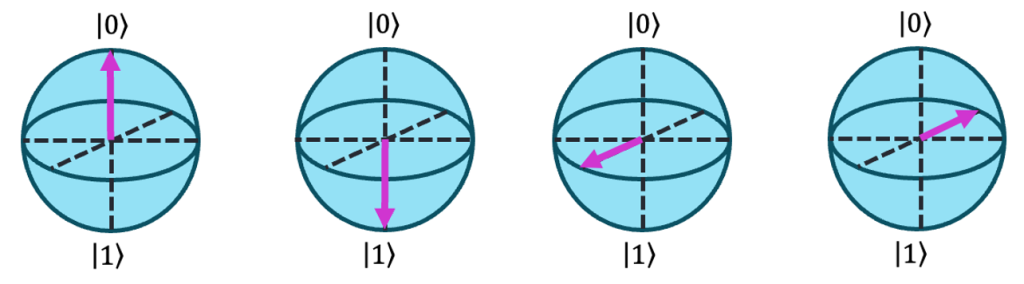
Imagine a unit sphere with a vector pointing from the origin to a point on its surface. This vector corresponds to the state of the qubit. For example, the classical states ∣0⟩ and ∣1⟩ sit at the north and south poles of the sphere (i.e., +1 and −1 on the z-axis), while any pure superposition state lies somewhere on the surface in between [3]. Several examples can be seen in Fig. 2.

Figure 2: representation of different quantum states on Bloch sphere. From left to right: \(|0 \rangle \), \(|1 \rangle \),  \(\frac{1}{\sqrt{2}} \left( |0 \rangle + | 1 \rangle \right) \), \(\frac{1}{\sqrt{2}} \left( |0 \rangle – | 1 \rangle \right) \)

Now, there’s a small catch with this representation. These pictures show the quantum state at a fixed moment in time, but they don’t capture how the state evolves. As we derived earlier, a superposition state like \(\frac{1}{\sqrt{2}} \left( |0 \rangle + | 1 \rangle \right) \) will precess around the z-axis at a frequency . This is a headache — constant rotation can make it hard to track state evolution over long protocols or gate sequences.

To resolve this, we perform a coordinate transformation into a rotating reference frame that spins at ​. In this rotating frame, the precession disappears, so a stationary superposition remains stationary, and the Bloch vector appears fixed. This makes it far easier to analyze qubit dynamics.

Unfortunately, real-world quantum systems do not remain in perfect superposition states forever. Over time, interactions with the environment cause the qubit to lose coherence and relax back to equilibrium. While the Bloch sphere gives us a perfect geometric picture of an ideal, isolated qubit, real systems gradually drift away from the surface of the sphere as they lose information. These mixed states, which describe statistical uncertainty or loss of coherence, fall inside the sphere, rather than on its surface.

There are two key timescales that characterize this behavior:

T₁​ (Energy relaxation time): The timescale over which the qubit relaxes from the excited state ∣1⟩ to the ground state ∣0⟩. This causes the Bloch vector to tip toward the north pole.

T₂ (Dephasing or coherence time): The timescale over which the relative phase between ∣0⟩ and ∣1⟩ becomes scrambled, due to fluctuations in the environment. This causes the Bloch vector to shrink toward the z-axis. Note that this is the intrinsic dephasing time, which we differentiate from the dephasing time commonly represented by , which we introduce later.

Together, these processes cause the qubit’s state to transition from a pure state (on the surface of the sphere) to a mixed state (inside the sphere). When fully decohered, the qubit no longer carries useful quantum information.

When the qubit is not being actively driven (see the next section), the dynamics of the system in the presence of decoherence/dephasing are described by the Bloch equations:

\(\frac{dx}{dt} = -\frac{1}{T_2}x\)

\(\frac{dy}{dt} = -\frac{1}{T_2}y\)

\(\frac{dz}{dt} = -\frac{1}{T_1}(z-z_\infty)\)

Here, x, y, and z are the components of the state vector: x and y describe coherence in the transverse plane, z is the population difference between ∣0⟩ and ∣1⟩ and z_∞ = +1 corresponds to the thermal equilibrium state (i.e., full population in ∣0⟩). In the next section, we’ll show how to coherently manipulate the qubit using an external drive field, rotating it around different axes of the Bloch sphere to implement quantum protocols.

Adding drive

Any type of qubit application, whether sensing or computation, needs to be able to manipulate the states of qubits on command. This allows users to both measure the quality of their qubits (via T₁ and T₂ measurement) and perform more complex gate sequences. To do this, we apply another oscillating electromagnetic field, with its direction of propagation defined along the x axis. If the frequency of this drive field matches the energy difference \(\omega_0\) between the two levels, we say that it is in resonance with the two-level system, and it will cause the quantum state to oscillate between 0 and 1, with a frequency dictated by the amplitude of the driving field.

We can write this field as

\(\widehat{H}_{drive}=\frac{\hbar \Omega}{2}\cos{(\omega_0 t + \phi)}\widehat{\sigma}_x\)    (4)

Let’s unpack a few key features. The quantity \(\frac{\hbar \Omega}{2}\) represents the power of the driving signal, but as with the Hamiltonian in Eq. 2 we typically write it in terms of frequency, which will eventually give us the Rabi frequency, or the speed with which the driving field flips the system between 0 and 1. Note that this value is different to (and often orders of magnitude smaller than) the frequency of the driving field itself. The operator \(\widehat{\sigma}_x\) is another Pauli matrix and indicates that the system is being driven about the x-axis of the lab frame. The values \(\omega_0\) and \(\phi\) are the frequency and phase of the drive field respectively. Note that the drive can be off-resonant from the two-level system, but here we’re examining the on-resonance case.
As with the Bloch sphere, to simplify the system dynamics, we shift into a rotating frame at frequency \(\omega_0\) This rotating frame co-moves with the qubit’s natural precession and eliminates the fast time dependence from the cosine term. In this frame, the Pauli matrix transforms as:

\(\sigma_x \rightarrow \cos{(\omega_0 t)} \sigma_x + \sin{(\omega_0 t)} \sigma_y\)

We’ll skip the detailed math here, but the effect is this: when the Hamiltonian is transformed into the rotating frame, it produces terms that vary slowly in time \((\omega \approx 0)\) and others that oscillate at \((\omega \approx 0)\), which are very fast. By applying the rotating wave approximation (RWA), a standard simplification in quantum optics and control, we drop these fast-oscillating terms because their effect averages to zero over the timescales of interest. The resulting effective Hamiltonian in the rotating frame is:

\(\widehat{H}_{drive,RWA}=\frac{\hbar \Omega}{2} \left( \cos{( \phi)}\widehat{\sigma}_x + \sin{( \phi)}\widehat{\sigma}_y \right)\)    (5)

This describes a slower rotation in the rotating frame, where the axis of rotation lies in the x–y plane and is controlled by the phase ϕ of the drive. If ϕ = 0, the rotation is purely about x; if ϕ = π/2, it is about y; and so on.

Rabi oscillations

As mentioned in the previous section, applying a drive field causes the system to oscillate between quantum states. Clever users can manipulate the parameters of the drive field duration and phase to rotate the state vector to any point of their choosing. One of the most fundamental tests of this behavior is the Rabi oscillation experiment, which demonstrates that the system behaves like a true two-level quantum system. It typically follows three steps, illustrated in Fig. 3:

Step 1: Initialize the qubit. This can be done by actively resetting the qubit to zero, or simply waiting for a few T1 cycles, provided T1 is a short enough.

Step 2: Apply a Rabi pulse. A drive field is applied along the x- or y-axis for a time T. This pulse causes the state vector to rotate on the Bloch sphere.

Step 3: Read out the qubit. After the Rabi pulse, the system is immediately measured.

The experiment is repeated with increasing pulse lengths, sweeping the state through a range of superpositions between ∣0⟩ and ∣1⟩, and then eventually back to ∣0⟩. But remember: quantum measurements can only return 0 or 1, never “halfway” values. To build up a meaningful picture of the state, each pulse duration is repeated many times, typically thousands, to extract a probability of measuring ∣1⟩.

Figure 3: Rabi sequence and typical data distribution. Top left: a Rabi sequence consists of a single pulse of length τ applied to the qubit, after which the state is immediately measured. Top right: the qubit is initialized into the ground state and is driven around the x-axis of the Bloch vector to some arbitrary superposition state. Bottom: to obtain the full picture of the state, the measurement is repeated 1000 times for each value of τ. π and π/2 pulse lengths are indicated in red. Note that the envelope of the oscillation also decays.

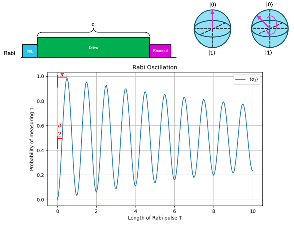
Driving the system for a long time will cause spin to decohere, or in Bloch sphere terms the vector will begin to shrink back toward the origin. This can be seen in Fig 3, where the system gradually fails to fully return to ∣1⟩ or ∣0⟩, eventually settling into a disordered state with no useful quantum information.

Typical values of interest for a Rabi measurement are the lengths of the driving pulses that cause the system to flip from 0 to 1 (a π-pulse) and from 0 to an equal superposition state (a π/2-pulse). After these values are determined, more complex pulse sequences can follow, which we will explore in the following section.

Ramsey and CPMG sequences

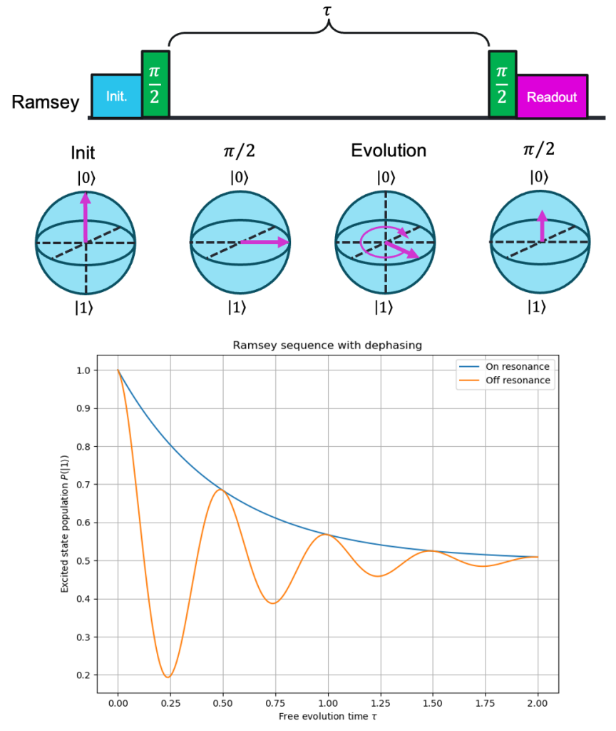
With the knowledge of our π- and π/2-pulse lengths in hand, we can now move on to quantifying the coherence time. The first test is to measure how long a qubit in a superposition state can retain its phase information, a process known as Ramsey interferometry. Like with the Rabi sequence, we always start with a qubit that has been initialized into the ground state ∣0⟩. A π/2 pulse rotates the state from +z into the x-y plane, creating a 50/50 superposition. Right after this happens, we allow the state to evolve freely for a time τ. According to the Bloch equations, the state vector will begin to shrink back toward zero due to decoherence (\(T_2\)). However, there is another process that happens on a much faster timescale. Due to influence from the environment, such as magnetic field fluctuations or small detunings (i.e., drive frequencies offset from resonance), the state vector will begin to rotate around the z-axis as the fragile quantum state becomes disrupted. This phenomenon is known as dephasing. We didn’t intentionally cause the qubit to precess, but these random fluctuations accumulate phase anyway.

To detect this accumulated phase, we project the qubit’s state back onto the measurement axis. This is done by applying a second π/2 pulse, which converts the x–y plane phase shift into a measurable population difference along z. If there were no dephasing, this would result in the qubit being placed in the ∣1⟩ state. As seen in Fig 4, when you repeat the Ramsey sequence for various free evolution times τ and measure the probability of finding the qubit in state ∣1⟩, you observe an oscillating signal, determined by the detuning of the drive signal and the true qubit resonance [4]. These oscillations are bounded by an exponential envelope, reflecting how coherence is lost over time and characterized by \(T_2^*\), the dephasing time.

These measurements are often repeated thousands of times per value of τ, and the resulting data points form a cosine signal decaying to 0. Fitting this envelope gives you a direct measure of \(T_2^*\), which includes both intrinsic decoherence and low-frequency noise (e.g., slow drifts in magnetic fields or qubit frequency).

Figure 4. Ramsey interferometry. Top: a Rabi sequence consists of two   pulses separated by free evolution time Middle: The state vector precesses around the z-axis during free evolution and is projected back onto the z-axis before measurement. Bottom: the measurement is repeated many times for each value of . The excited state will gradually decay as , with oscillations introduced by driving with an off-resonant signal.  

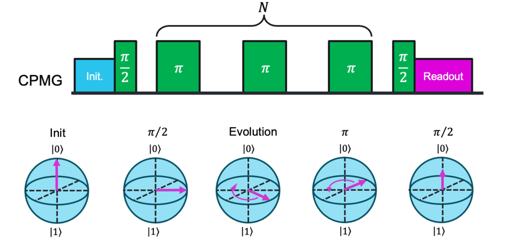
While Ramsey sequences provide a powerful way to measure a qubit’s dephasing time ​, this value includes both intrinsic decoherence and slow, reversible noise sources like low-frequency magnetic field drift and is not the “true” T₂​ as represented in the Bloch equations. To isolate the qubit’s intrinsic coherence time, we can apply a spin echo or Carr-Purcell-Meiboom-Gill (CPMG) sequence. These techniques begin similarly to a Ramsey sequence but insert additional π pulses at precise intervals during the free evolution period. Each π pulse flips the state vector about the x- or y-axis, reversing the direction of phase accumulation and effectively canceling out errors from slow fluctuations. These pulses can be repeated dozens or even hundreds of times, with the length and spacing of the π-pulse train determining the range of environmental noise frequencies that are effectively suppressed. The result is a slower decay of coherence, allowing us to measure the intrinsic T₂ of the system, a more meaningful benchmark for applications that demand sustained quantum control. See Fig 5 for an example CPMG sequence.

Figure 5. CPMG sequence. After the initial  pulse, a series of equally-space  pulses rotate the vector around the x- or y-axis. This causes the direction of rotation to reverse, effectively erasing the phase accumulated between  pulses. After projecting back into the z-axis, a much more accurate picture of T₂ can be determined.

Performing Computation and Sensing Experiments

The sequences we’ve described: Rabi, Ramsey, and CPMG, form part of a standardized toolbox for evaluating the quality of qubits across all quantum platforms. Rabi and Ramsey measurements, in particular, are often repeated at different detuning to help pinpoint the precise resonant frequency of the qubit. Once this frequency is identified, the next priority is assessing how well the qubit holds its state. Long coherence times (T₁ and T₂) are critical, as they allow for longer and more complex manipulations.

In quantum computing, qubit manipulation is performed using carefully timed pulses, most often π and π/2, which rotate the state vector in controlled ways. These rotations are typically grouped into standard operations called quantum gates. For instance, a Hadamard gate rotates the state vector from the +z direction (|0⟩) to the +x direction, and can be implemented using a π/2 pulse about the y-axis followed by a π pulse about x. More advanced gates, especially those involving two qubits, are beyond the scope of this paper, but the principle remains the same: quantum algorithms are executed by applying sequences of pulses that steer qubits around the Bloch sphere.

In quantum sensing, the weaknesses of quantum systems, namely their sensitivity to environmental noise, is turned into a strength. Here, pulse sequences are typically simpler and are intentionally designed to allow the qubit to interact with its environment. Deviations from expected behavior, due to a magnetic field or an electric gradient, are then interpreted as signals.

For example, if a qubit in a known DC magnetic field is exposed to an additional, unknown field, this will alter the energy splitting between its states. As a result, a drive signal that was once resonant may now be slightly off resonant, causing the qubit to accumulate a different phase during free evolution. By performing a Ramsey measurement before and after the auxiliary field is applied, this phase shift, and hence the strength of the unknown field, can be inferred. Repeating this process many times, using high-quality qubits with long coherence times, allows quantum sensors to achieve measurement precision far beyond what’s possible with classical techniques.

Implementing Pulse Sequences in Hardware

All the pulse sequences described in this paper, whether for Rabi oscillations, Ramsey interferometry, or CPMG coherence measurements, ultimately require precise, programmable control of the qubit. While the exact parameters of the pulse highly depend on the choice of qubit, the base physics are the same. In this section we talk about a few different implementations of pulse sequences using Moku.

Superconducting qubits are typically manipulated by IQ-modulated microwave pulses. An arbitrary waveform generator (AWG) produces low-frequency or DC pulse envelopes, known as basebands. These basebands are combined with a high-frequency local oscillator using an IQ mixer (digital or analog) to generate microwave pulses with tunable amplitude, frequency, and phase. The relative amplitude and timing of the “I” and “Q” channels control the final pulse’s rotation axis and phase on the Bloch sphere. Pulse shapes, often Gaussian, are chosen for optimal control and minimal spectral leakage.

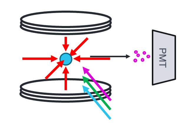
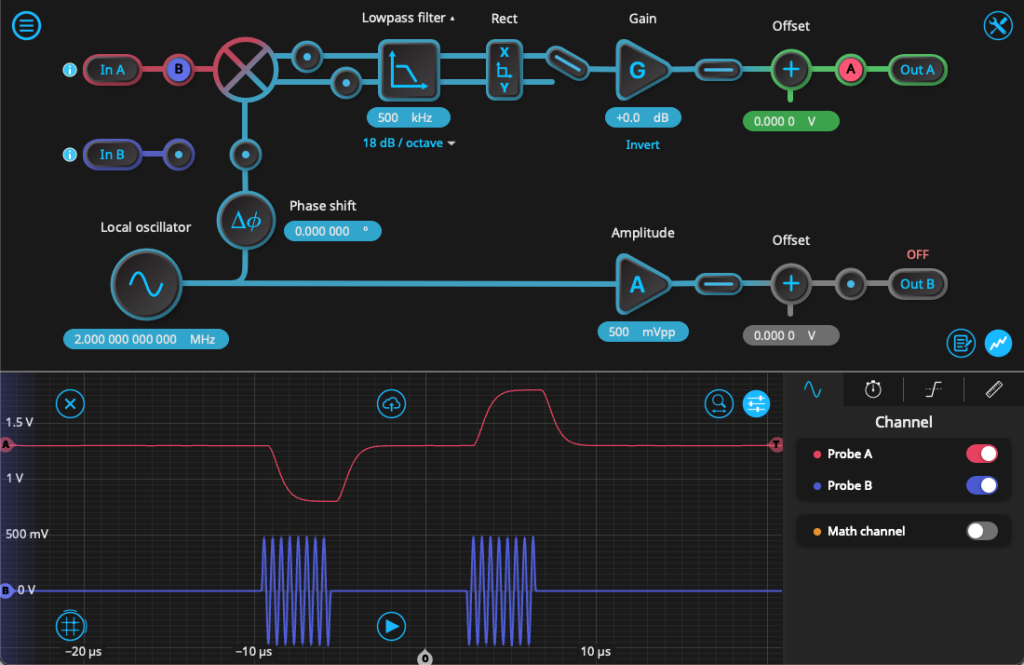
In optical qubit platforms like trapped ions or neutral atoms, pulse control is commonly achieved using acousto-optic modulators (AOMs). Here, an RF signal generated by an AWG drives the AOM, which modulates the amplitude, frequency, or phase of a laser beam. This setup allows for high-speed optical gating with precise control over timing and rotation angle, enabling qubit operations such as π and π/2 pulses (see Fig. 6).

Figure 6. Top: the Moku Arbitrary Waveform Generator supports a variety of preset functions, as well as the option to upload custom waveforms via .csv file or mathematical function. Bottom: Two modulated, in-phase RF pulses (2 MHz) generated by the Moku Arbitrary Waveform Generator and captured by the Oscilloscope. Such a sequence could be used to drive an AOM.

The Moku Arbitrary Waveform Generator, one of many instruments available on the reconfigurable Moku platform, enables users to generate these signals with ultra-stable clock precision and highly flexible waveform synthesis. It supports sine waves, Gaussian envelopes, and fully custom waveforms, either uploaded via .csv or defined by an equation. In superconducting qubit setups, two synchronized channels can be used for I and Q control, while in atomic systems, baseband or modulated RF outputs can be used to drive AOMs. The Arbitrary Waveform Generator also includes a variety of triggering options for synchronizing sequences with other equipment, including a TTL input and a manual triggering option.

Moku also offers a number of other software-defined instruments to assist with pulse generation. Users can debug pulses with the Moku Oscilloscope and Spectrum Analyzer, deployed in Multi-Instrument Mode for viewing in both the time and frequency domains in real time. The Oscilloscope can help users confirm pulse shaping and timing across multiple input channels, whereas the Spectrum Analyzer can ensure that there is no distortion or added harmonics in frequency space.

While not covered in this white paper, pulses are often demodulated after capture to determine the qubit state, which is typically encoded in the phase of often coherent signals – for example, reflected microwave pules or modulated photocurrents. The Moku Lock-in Amplifier adds the capability to perform dual-phase demodulation with perfect synchronization, as the local oscillator (LO) shares the system clock with the Arbitrary Waveform Generator, allowing for microradian precision. Users can view and output both I and Q quadrates and capture data traces directly from the embedded Oscilloscope, eliminating the need for a digitizer. Moreover, I and Q outputs can be fed to Moku Cloud Compile modules for post-processing, such as boxcar averaging or decimation. See Fig. 7 for an example of a pulse sequence demodulation.

Figure 7. Demodulation example. The RF input (Probe B) shows a Ramsey-like sequence with the second pulse shifted by 180°. After demodulation with a 2 MHz local oscillator and filtering, the output X quadrature is shown at Probe A. The phase shift between the two pulses is clearly seen in the DC baseband signal.

Often, when converting between analog and digital signals through ADCs and DACs, signals are often distorted by the addition of harmonics or spurs, so proper filtering is essential to quantum experiments. The Digital Filter Box can assist in cleaning up these signals, allowing users to program different filter shapes, functions, and cutoff frequencies. Deploying together with other instruments in Multi-Instrument Mode, the Digital Filter Box can receive input signals from the analog frontend and prefilter them before passing to the Lock-in Amplifier for demodulation.

Moku also offers robust Python and Matlab APIs for coordinating complex experiments, automating pulse generation and data trace collection, and parameter sweeping (such as the value  in a Ramsey experiment). No SCPI commands or common VISA libraries are needed to integrate Moku into a given setup – users can just import, connect, and configure.

With its reconfigurable, software-defined architecture, Moku makes it easy to prototype, tune, and deploy pulse sequences as experimental demands evolve.

Conclusion

In this white paper, we’ve walked through the essential physics of two-level quantum systems, using the Bloch sphere as a visual foundation. We introduced Hamiltonian formalism and time evolution, discussed how real-world systems experience decoherence through mechanisms like energy relaxation and dephasing, and explored how rotating frames and driven fields enable coherent control. From there, we covered basic pulse sequences such as Rabi, Ramsey, and CPMG that are used to characterize and manipulate qubits. Lastly, we showed how these pulse sequences could be physically implemented with the Moku Arbitrary Waveform Generator. Together, these tools form the groundwork for both quantum computation and quantum sensing.

References and Footnotes

[3] Why is the lower energy state on top? It’s a convention inherited from the NMR community. Typically, the magnetic field is defined to run along the +z axis, meaning that the lower energy state occurs when the vector is aligned with +z, and higher energy when it is anti-aligned.

[4] Initially, qubit resonance frequencies are often estimated based on device parameters or calibration data. Ramsey interferometry provides a precise method to determine the true resonance frequency by observing the oscillation frequency as a function of detuning.