Dual-frequency resonance tracking (DFRT)

Real-time resonance tracking is important in a range of applications, from microelectromechanical systems (MEMS) based inertial sensing to atomic force microscopy (AFM). This application note compares two methods of tracking resonances: one utilizing a phase-locked loop (PLL) and the other utilizing dual-frequency resonance tracking (DFRT). While the PLL method works well in most conditions, it can struggle with the abrupt phase shifts experienced under critical coupling. DFRT overcomes this difficulty with amplitude-dependent feedback control, providing a more reliable solution.

Here, we demonstrate DFRT by combining dual Lock-in Amplifiers and a PID Controller on a single Moku:Pro device. Dual-frequency signals, generated by a two-channel Waveform Generator, were tested on a simulated resonator, with positive results demonstrating the utility of the technique in situations where PLL methods are less reliable.

Introduction

Two prominent techniques for achieving resonance tracking are the PLL method and DFRT. The PLL approach relies on monitoring the phase difference between the drive signal and the system’s response. By maintaining a constant phase difference, the drive signal is locked to the resonant frequency, which is useful in MEMS resonance tracking. Figure 1 illustrates the block diagram of a PLL system for resonance tracking, comprising a Moku Lock-in Amplifier, PID Controller, and Waveform Generator. Notably, the Moku Lock-in Amplifier includes embedded PID functionality, enabling resonance tracking with no additional instrumentation.

The Lock-in Amplifier demodulates the response signal, using the drive signal as a reference, to determine the phase difference between the two signals. This phase difference is then compared to the target phase offset, and the resulting error signal is processed by the PID Controller. The PID Controller generates a frequency tuning signal, which adjusts the Waveform Generator to continuously track the resonant frequency.

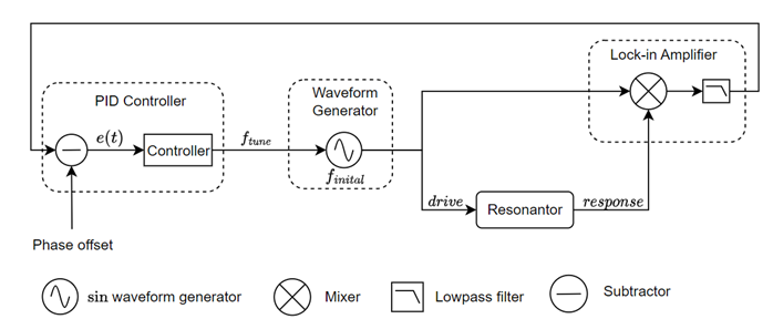
Figure 1: The PLL detects the phase difference between the drive and response signals, sending the phase difference to the PID Controller. The PID Controller then generates a control signal, 𝒇𝒕𝒖𝒏𝒆, which adjusts the Waveform Generator to tune the frequency and track the resonant frequency. 

For a PLL system to operate effectively, there should be a continuous phase relationship between the drive and response signals, as the drive frequency is varied. This makes PLL well-suited for MEMS gyroscopes, which typically operate in an over-coupled mode, as well as for certain AFM micro-cantilever sensors that function in under-coupled conditions. However, its performance is limited in critically coupled conditions. In this case, sweeping the frequency from to results in a sudden 180° phase shift at resonance. This abrupt change can disrupt the tracking process, potentially causing oscillations. Although such instances are uncommon, they can pose significant challenges when they occur. 

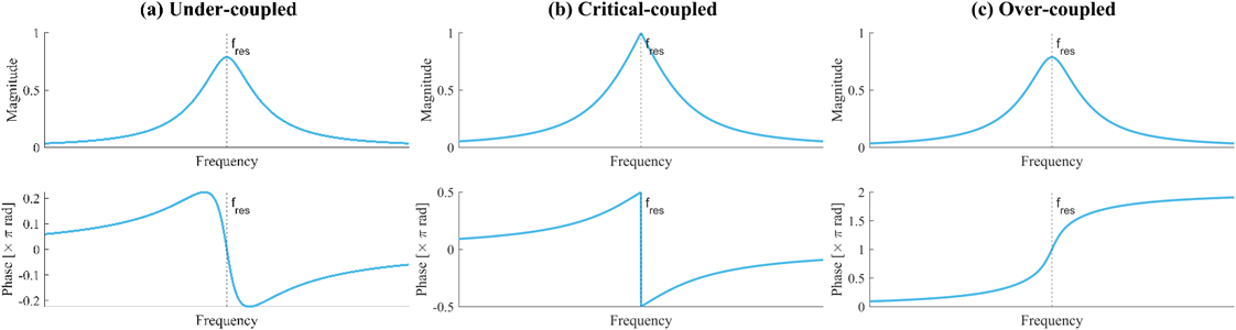
Figure 2: Resonance behavior can be categorized into three coupling conditions: under-coupled, critical-coupled, and over-coupled. In both under-coupled and over-coupled conditions, the phase change around the resonant frequency is linear and continuous. In the critical-coupled condition, a 180° phase shift is observed near . The resonance characteristics are derived from simulations of micro-ring resonator coupling systems.

Additionally, for reliable PLL functionality in AFM applications, the phase response of the system should remain stable at the resonator frequency while the cantilever is scanning. This stability is crucial because PLLs can only maintain a fixed phase difference — any variation in the phase response at the resonator frequency could lead to errors in tracking the resonator frequency. However, this may not be achievable under certain conditions, such as in piezo–response force microscopy, where the cantilever’s deflection signal exhibits a 180° phase flip between oppositely oriented domains based on their polarization alignment with respect to the drive electric field. The PLL method would not be able to track the correct resonant frequency, as the phase response isn’t stable. Therefore, the tracked resonant frequency would not be the correct frequency as the phase–to–frequency mapping relation changes while scanning different materials. For example, on the two sides of the domain walls, one side has a 90° phase difference at the resonant frequency, but the other side has a resonant frequency of -90°. To address these challenges, alternative resonance-tracking techniques, such as DFRT, become necessary.

Dual-frequency resonance tracking 

Effective PID control requires that the error signal exhibits opposite signs on either side of the central resonant frequency. This can be achieved by differentiating a symmetric signal, converting it into an antisymmetric form with the sign change necessary for precise feedback control. Figure 3 presents a comparison between the original and differentiated magnitude responses of an AFM micro-cantilever sensor. Studying the original magnitude response, it is not possible to determine the current frequency relative to the resonant frequency () from an isolated magnitude measurement — a single magnitude value corresponds to two distinct frequency values, one on either side of . In contrast, the differentiated response resolves this ambiguity: on the left side, where the frequency is below , the differentiated magnitude values are positive, while on the right side, where the frequency exceeds , the values are negative. This distinction enables more precise resonance tracking for PID control.

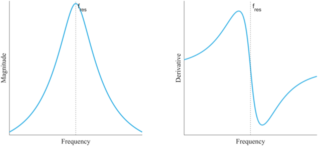
Figure 3: The original resonator magnitude response (left) is symmetric. In contrast, its derivative (right) generates an antisymmetric magnitude profile with opposite signs on either side of resonance, making it ideal for feedback control.

Similarly, dual-frequency resonance tracking operates on a principle analogous to the derivative, but with a fixed derivative step size of . The concept of dual-frequency tracking is illustrated in Figure 4. The amplitudes of the two tones depend on their proximity to the resonant frequency. If is closer to the resonant frequency than , the amplitude of tone would be larger than , and vice versa. Hence, the key would be to move the center frequency of and to make the center match the resonant frequency. An explanatory diagram is provided in Figure 5. As a result, the error signal remains at zero when the center frequency, , aligns with .

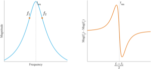
Figure 4: The resonance magnitude response is symmetrical around the center frequency. The frequencies and are separated by a constant frequency difference of and changeable center frequency of . The error signal is obtained by subtracting the magnitudes of two frequency components.

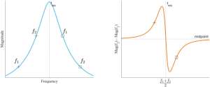
Figure 5: This figure illustrates two scenarios. The “+” denotes cases where the center frequency, , is lower than the resonator frequency, . Conversely, the “☐” indicates cases where the center frequency exceeds . The resulting response, , shows “+” above the midpoint and “☐” below the midpoint. Consequently, the PID Controller can adjust the center frequency to align with the resonator frequency as needed.

Implementation on Moku:Pro

Two Lock-in Amplifiers are required to detect the amplitudes of the two frequency components in the input signal, with the PID Controller performing subtraction to stabilize the system. The principle of dual-frequency resonance tracking is shown in Figure 6. In this setup, two sine waveforms are generated using a Waveform Generator, combined via a signal combiner, and then applied to the resonator. The amplitudes of the two frequency tones are then measured and fed into a PID Controller to enable resonance tracking.

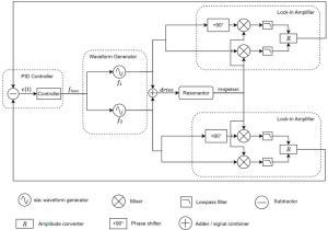
Figure 6: Block diagram of a dual-frequency resonance tracking setup. Two frequency components, and , are generated by independent sine waveform generators and combined using an analog signal combiner before being sent to the resonator. Both frequency components are demodulated by dual-phase demodulators, and the amplitudes of each tone are calculated. The difference, , between the two amplitudes is then sent to the PID Controller for frequency tuning and resonance tracking.

Figure 7 illustrates the implementation of DFRT using Multi-instrument Mode on Moku:Pro. In this setup, two Lock-in Amplifiers (one in Slot 1 and the other in Slot 2) are used to measure the amplitudes of the two frequency components. The amplitude signals are sent to a PID Controller in Slot 3, which generates a feedback control signal. This control signal frequency modulates the Waveform Generator, allowing it to adjust the center frequency and track the resonance effectively. The two channels of the Waveform Generator are sent separately to two Lock-in Amplifiers as reference signals. 

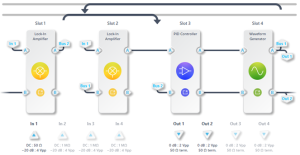
Figure 7: A Moku:Pro configured for resonance tracking. The two-channel Waveform Generator is set up as a frequency modulated sine generator, with the PID Controller’s control signal used to tune the center frequency. The error signal is generated by subtracting the outputs of the two Lock-in Amplifiers.

The Waveform Generator configuration is shown in Figure 8. The Waveform Generator produces two frequency components using separate channels set at 10 MHz and 11 MHz, creating a frequency difference of 1 MHz between them ( MHz). Both channels have a frequency modulation depth of 1 MHz/V and are modulated by the same input signal, Input A. This ensures that both channels are modulated equally, maintaining a consistent 1 MHz frequency difference between them. These two signals are then sent to two Lock-in Amplifiers, where they are used as reference signals to demodulate the response signal from the resonator.

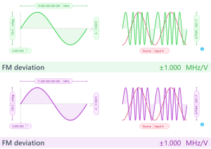
Figure 8: The two-channel waveform generator is set up with sine wave generators at 10 MHz and 11 MHz. The frequency modulation depth of both channels is configured to 1 MHz/V, ensuring a consistent modulation of both tones.

The configuration of the Lock-in Amplifiers (both identically configured) is shown in Figure 9. The Lock-In Amplifier features an internal PLL which locks its local oscillator to the signal received on In–B (the Waveform Generator output). The PLL in the Lock-in Amplifier is used only for generating the demodulation reference and does not contribute to resonator frequency tracking. To reduce interference from adjacent frequency components, the Lock-in Amplifiers’ lowpass filter is set to 100 Hz with an 18 dB/octave slope. Notably, the low-pass filter’s corner frequency should be adjusted to align with the AFM scanning rate or signal bandwidth in the experiment. If the scanning rate exceeds the filter’s response time, amplitude and resonator frequency transitions may not be accurately tracked. The Lock-in Amplifier measures the amplitude of the corresponding frequency components in the In-A signal (resonator response) and outputs the result through Out-A. 

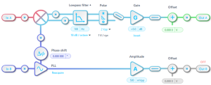
Figure 9: Lock-in Amplifiers’ configuration. The demodulation reference is derived directly from the Waveform Generator output. The lowpass filter is configured with a 100 Hz corner frequency and an 18 dB/octave roll-off. The amplitude of In-A (the tone as measured in the resonator’s response) is sent to Out-A. 

The error signal is obtained by subtracting the outputs of the two Lock-in Amplifiers, with this operation carried out by the control matrix in the PID Controller (see Figure 10). To minimize the error signal, the PID Controller is configured as a proportional-integral (PI) controller. The integrator eliminates the DC error signal. The integrator’s zero-crossing point can be adjusted to meet experimental requirements. Increasing the integrator crossover frequency allows for faster resonance tracking but may reduce phase margin, potentially causing unwanted overshoot or oscillations. 

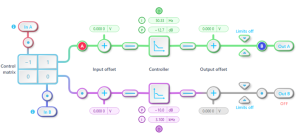
Figure 10: The error signal is generated by the control matrix (In-B – In-A), which is then sent to the PID Controller. The PID Controller is configured with a proportional gain of -12.7 dB and an integrator with a crossover frequency of 50.33 Hz. 

In this experiment, the resonator is simulated using a bandpass filter with a variable center frequency, causing the amplitudes of the two frequency tones to change according to the center frequency of the filter. The device connections and FIR filter configuration are shown in Figures 11 and 12, respectively. The center frequency of the FIR filter is tuned to assess the performance of DFRT. 

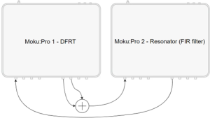
Figure 11: Device and BNC cable connections are as follows: Moku:Pro 1 is used for resonance tracking, while Moku:Pro 2 simulates a resonator using an FIR filter. The FIR filter is configured as a bandpass filter with a variable center frequency. Two frequency tones generated by Moku:Pro 1 are combined using an analog signal combiner. 

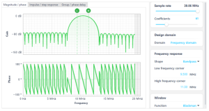
Figure 12: The FIR filter is configured as a bandpass filter with a 39.06 MHz sampling rate and 61 coefficients. The center frequency is set to 10 MHz and can be tuned to evaluate the resonance tracking performance. 

Finally, resonance was successfully locked using DFRT. The user interface of the PID Controller, shown in Figure 13, displays the control signal output. The FIR filter’s center frequency was tuned from 10.5 MHz to 11.5 MHz in 0.25 MHz steps. Each step in the PID output corresponds to a control signal change of approximately 250 mV, which translates to a 0.25 MHz frequency modulation. It is important to note that the step size does not precisely match 250 mV, as the FIR bandpass filter’s response curve is not perfectly symmetric around the center frequency. This mismatch also reflects the behavior of real resonators, which may exhibit similar magnitude response irregularities. This can be compensated for, if needed, by introducing an input offset in the PID Controller. 

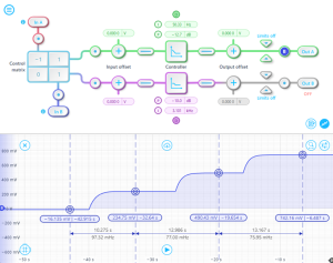
Figure 13: The PID Controller user interface, the blue line plots the output control signal. The markers in the figure indicate the control voltages. Each step in the control signal is approximately 250 mV, corresponding to a 0.25 MHz frequency tuning. The actual step size does not exactly match 250 mV due to the FIR filter’s imperfect symmetry. 

Summary

This study introduces two key techniques for real-time resonance tracking, important for applications like MEMS inertial sensors and atomic force microscopes: PLL and DFRT. The PLL approach works well for over- and under-coupled systems by maintaining a constant phase difference between the drive and response signals. However, this method faces challenges in critically coupled conditions due to abrupt 180° phase shifts, which can disrupt tracking. Additionally, it is less effective when the phase response is influenced by the material being tested.

To address this, DFRT uses dual-frequency signals to determine the resonant frequency, enabling precise feedback control through a PID controller. Successfully implemented on Moku:Pro, the DRFT effectively tracks frequency deviations in a resonator simulated with an FIR filter. It is worth noting that Moku:Pro DFRT focuses solely on tracking and does not measure the resonator’s amplitude or phase response at . Obtaining these response characteristics requires additional Moku hardware devices.

The results show that DFRT achieves stable and accurate resonance tracking, with real-time adjustments compensating for resonator asymmetries. This establishes DFRT as a viable alternative to the PLL method, particularly in scenarios where critical coupling or material variations compromise PLL method performance. By utilizing the amplitude response as the error signal, DFRT enhances tracking accuracy and robustness in such conditions.

References 

[1] B. J. Rodriguez, C. Callahan, S. V. Kalinin, and R. Proksch, “Dual-frequency resonance-tracking atomic force microscopy,” Nanotechnology, vol. 18, no. 47, p. 475504, Nov. 2007, doi: 10.1088/0957-4484/18/47/475504.