To create a neural network, this step-by-step example uses sum.ipynb, where the expected output is simply the sum of the inputs and uses only one hidden layer. While this simple operation can be completed in many ways, it’s easy to train the Moku Neural Network to implement almost any function, from simple algebra to complex inference. Find other examples here and download the Neural Network guide here.
General prerequisites
To begin using the Moku Neural Network, you will need the following:
- A Moku:Pro device (Moku:Lab and Moku:Go are not currently supported)
- Moku Version 3.3, available for download on Windows or macOS
- A Python installation (v3.11); see our Moku Python installation guide for details. You can also install a navigator such as Anaconda. Your Python installation must be v3.11 or higher. If you’re unsure what version you have, check your Python version in a command prompt or terminal with Python –version or python3 –version.
Python prerequisites
After you have installed Python on your machine, run the following command to install the Moku Neural Network API into a command line or terminal window on your computer. This will install the API and pull in all required dependencies:
pip install 'moku[neuralnetwork]'
This should install the following:
- Moku Neural Network API
- Numpy 1.26.4
- Ipykernel 6.29.5
- Matplotlib 3.9.2
- Tqdm 4.66.5
- Tensorflow 2.16.2
- SciPy (required for this example, but not in general)
If you use Python regularly, it’s likely that most of these packages are already installed. To verify, open a command prompt or terminal and type pip install X, where X is the name of the package you want to install. If the package is already installed, the command will return a message as follows:
(base) jessicapatterson@Jessicas-MacBook-Pro ~ % pip install numpy

Requirement already satisfied: numpy in /opt/anaconda3/lib/python3.12/site-packages (1.26.4)
The procedure for installing tensorflow can vary depending on whether you want to use your GPU for calculations. For precise instructions on how to install, see Tensorflow’s documentation, especially if you foresee using a GPU. For now, simply use pip install tensorflow to confirm that it has been installed.
(base) jessicapatterson@Jessicas-MacBook-Pro ~ % pip install tensorflow
Once installed, try calling Tensorflow and creating a tensor, using this command:
(base) jessicapatterson@Jessicas-MacBook-Pro ~ % python -c "import tensorflow as tf; print(tf.reduce_sum(tf.random.normal([1000, 1000])))"
If this command executes with no error, the installation is complete and you can move onto the next step. If it returns the error “The TensorFlow library was compiled to use AVX instructions, but these aren’t available on your machine,” then your computer unfortunately cannot run Tensorflow. Please see their documentation for solutions to this issue.
(base) jessicapatterson@Jessicas-MacBook-Pro ~ % python -c "import tensorflow as tf; print(tf.reduce_sum(tf.random.normal([1000, 1000])))"

tf.Tensor(258.68292, shape=(), dtype=float32)
Training a simple neural network
For our first neural network, we will train a model to generate the weighted sum of the input channels with an optional bias/offset term. The weights and biases will be determined through artificial training data created in Python. We can then load the parameters onto the Moku Neural Network instrument and validate the model using the Moku Oscilloscope and its built-in Waveform Generator. This example will use a Jupyter notebook for easy, interactive execution of the Python code. However, a simple Python script written and executed from your favorite IDE will also suffice.
Begin by launching Jupyter from the Anaconda window, then upload and open the sum.ipynb Python notebook.
Step 1: Imports and function definitions
Start by running the first code block (Figure 1), which will import all necessary dependencies, as well as make a call to the neural network API. If the first block of code executes without error, then all of the pieces are in place and we can proceed to the next step. If an error returns, check the section above to make sure all the prerequisites are installed.
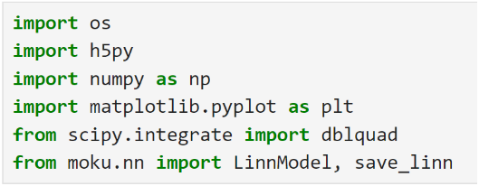
Figure 1: Required imports for sum.ipynb
Next, generate signals for training as shown in Figure 2. We need three input channels and one output channel of simulated data. You can also use your Moku:Pro to generate or capture real-world training data. Verify your training data by plotting our generated input signals alongside the desired, summed output (Figure 3).
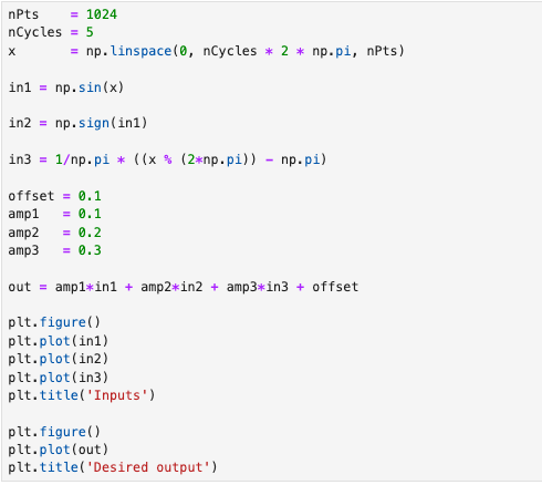
Figure 2: Generating simulated training data.
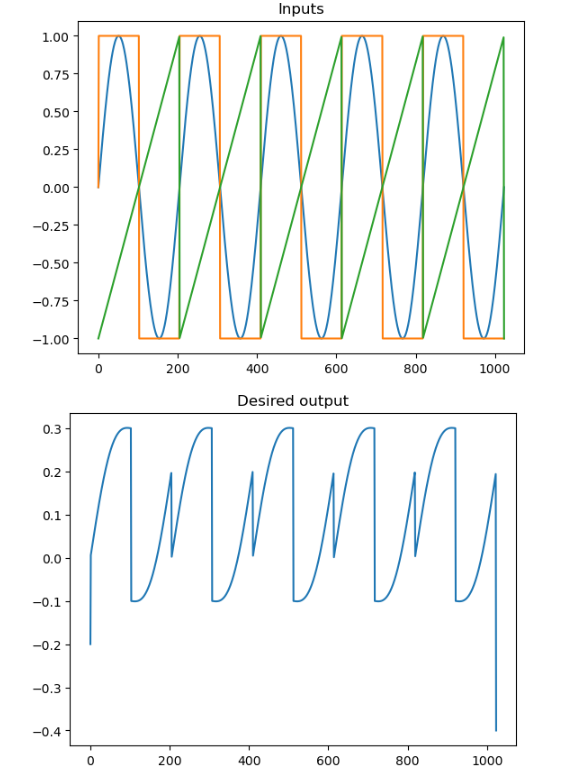
Figure 3: Simulated training inputs and desired outputs for training the model.
Next, we must prepare our data for training the model. We first reshape the inputs to a matrix of form (N,3) and the outputs to form (N,1) before sending them to the model. This code is shown in Figure 4.
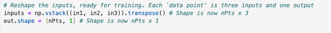
Figure 4: Transposing the data for training.
In this example, our existing data is sufficient for training, but you can choose to generate additional training data or scale the inputs and outputs. If you do choose to apply scaling, you will need to apply the same scaling in the Moku Neural Network at runtime.
Step 2: Define the model
We can now build the neural network model. We first create an object, entitled “linn_model,” which represents the Moku Neural Network instrument’s configuration and constraints. Once we have instantiated the model object in Figure 5, we can pass the training data previously generated into the model.
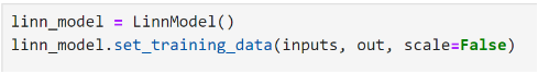
Figure 5: Instantiating the model.
We then define the model by creating an array, where each element in the array corresponds to a layer of the neural network. These elements are tuples, which give the number of neurons and the activation function for that layer. For example, (16, ‘relu’) indicates a layer of 16 neurons with a ReLU activation function. Other than the input and output layers, the number of neurons and activation function for each layer is up to the user to determine. While the sum.ipynb model uses a single neuron (Figure 7), feel free to comment out that model definition and try some of the additional options. You can have different activation functions and numbers of neurons for each layer.
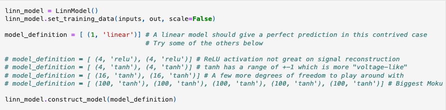
Figure 6: Constructing the model definition.
Executing this cell will populate the model definition, shown in Figure 7.
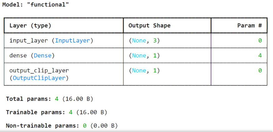
Figure 7: The sum.ipynb model definition.
When you create your own models, you can include up to five dense layers, also known as hidden layers, of up to 100 neurons each. Choose between ReLU, tanh, softsign, linear, and sigmoid activation functions for each layer. The layer outputs are passed through this activation function before moving to the next layer. Without these, the neural network operations would be entirely linear and collapse down to a single operation.
Step 3: Train the model and view feedback
Now that we have defined our model, we need to train it so that it will represent our desired mapping. This is as simple as calling the fit_model() function with a few basic arguments. We will allow our model to train for 500 epochs (training steps) and will hold aside 10% of our training data from above for validation. We also set an early stopping configuration to cease training when the loss functions plateau. This approach helps to avoid “overfitting,” where the model becomes very good at predicting training data at the cost of generality. It also has the benefit of speeding up the time to completion.

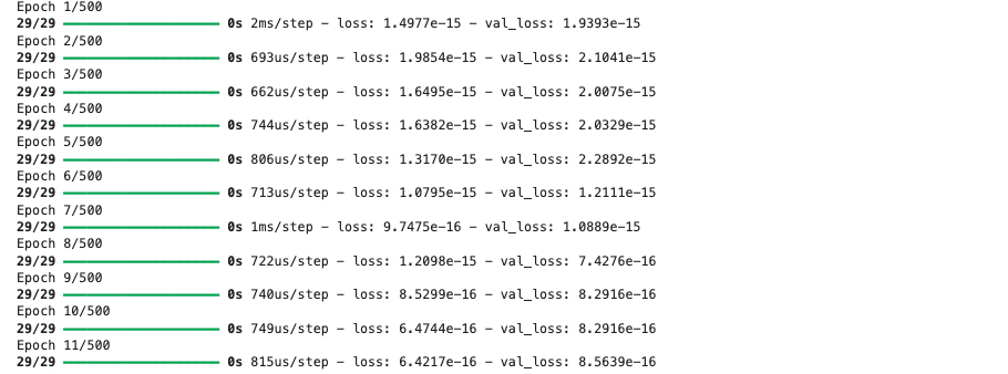
Figure 8: Training the model.
Once training is complete, plot the training loss and validation loss to assess the success of the training. Note that the loss in Figure 9 decreases as training goes on, which is expected.
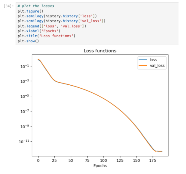
Figure 9: Plotted loss and validation loss from training.
You can choose to validate your model by plotting the predicted output now that it has been trained, as shown in Figure 10. Note the scale of the second plot showing the very small difference between the predicted and desired outputs.
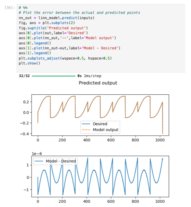
Figure 10: Plotted desired and predicted outputs from the model.
Step 4: Save the parameters
Now that we have a fully trained model, it’s ready to run on Moku. Save the model to a .linn file for use in the Moku Neural Network (Figure 11).

Figure 11: Function to save the network model to a .linn compatible with the Moku Neural Network.
Deploying and validating the model with Moku
In Multi-Instrument Mode on Moku:Pro (Figure 12), place a Moku Neural Network in Slot 1 and an Oscilloscope in Slot 2. Next, connect the outputs of the Oscilloscope to the inputs of the Neural Network. Then click “apply changes” and wait for the FPGA to configure.
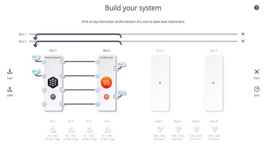
Figure 12: Multi-Instrument Mode configuration on Moku:Pro.
Now, open the Neural Network menu and upload the sum.linn file generated by the Python script using the “Load network configuration” button, located below the diagram as shown in Figure 13. You should see one layer with three inputs, one output, and a linear activation function, as expected.
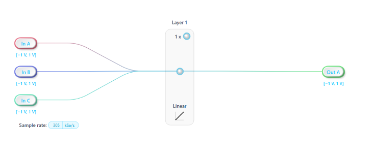
Figure 13: The Moku Neural Network with sum.linn loaded.
Enter the Oscilloscope and open the embedded Waveform Generator by clicking on the sine wave icon in the lower right corner. Generate two signals to test the model’s functionality, shown in Figure 14. For this example, we will use two sine waves: one with a 1 Vpp amplitude and 1 kHz frequency, and one with a 500 mVpp amplitude and 100 Hz frequency.
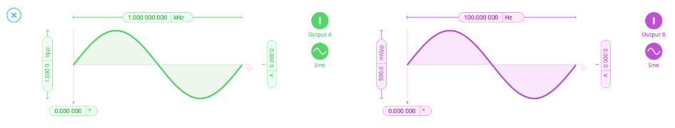
Figure 13: Embedded Waveform Generator example settings.
You should see the summed signal appear on Channel A of the Oscilloscope. Scale the Oscilloscope view with your mouse to view the signal. The two sine waves added together should resemble the signal in Figure 15.
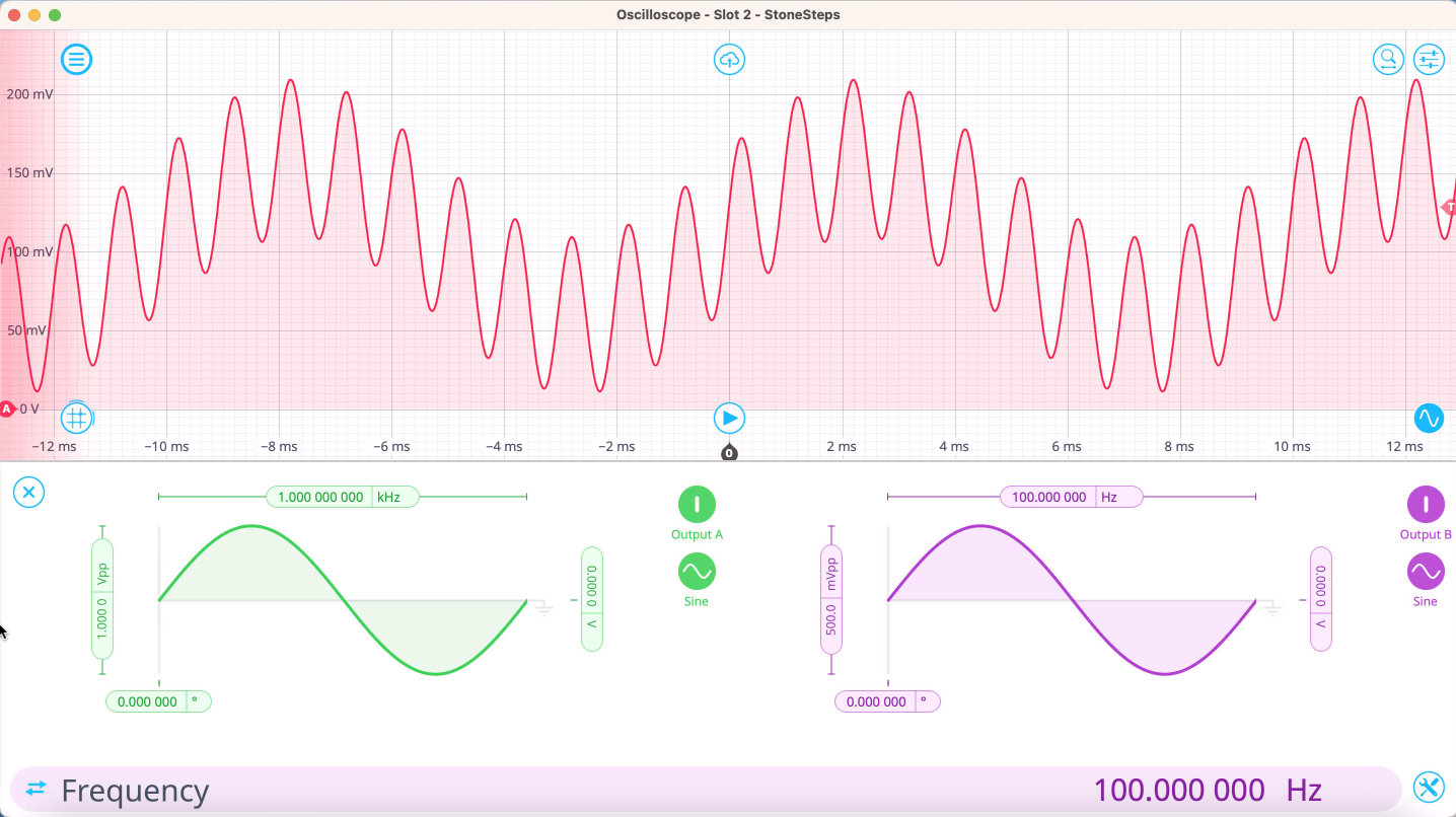
Figure 15: Output of the Moku Neural Network.
Verify operation of the network using cursors and built-in measurements as seen in Figure 16, testing for the expected amplitude and frequency components, or use the Moku Spectrum Analyzer. Feel free to test the network with additional signal types, frequencies, or other parameters.
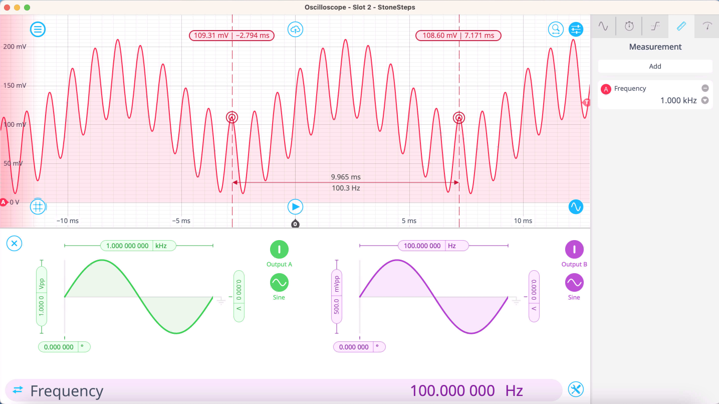
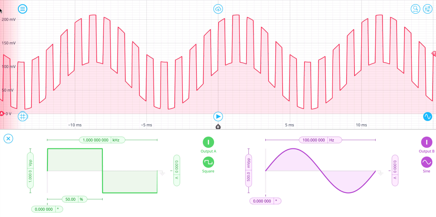
Figure 16: Verifying the Moku Neural Network output.
Conclusion
From here, you can modify the provided example scripts or write your own to create unique, powerful machine learning models to integrate with any other Moku instruments. Run control systems in real time, predict experiment outputs, and more, all with the only FPGA-based neural network integrated with a reconfigurable suite of high-performance test and measurement instruments.
Prefer a video tutorial? Watch our webinar on demand. You’ll learn how to implement an FPGA-based neural network for fast, flexible signal analysis, closed-loop feedback, and more.
Learn more about the Moku Neural Network
Review the rest of the provided examples, review specification, and continue learning about the Moku Neural Network. Have questions? Reach out to us here.
Join our User Forum to stay connected
Want to request a new feature? Have a support tip to share? From use case examples to new feature announcements and more, the User Forum is your one-stop shop for product updates, as well as connection to Liquid Instruments and our global user community.