Originally formulated to assess the stability of oscillators in atomic clocks, Allan variance provides a robust measure of frequency stability over varying timescales, which statistics such as standard deviation do not take into account. Allan variance can be performed using the Moku, an FPGA-based device that houses a reconfigurable suite of test and measurement instruments. Leveraging the unique Phasemeter instrument, one can record ultra-precise phase, frequency, and amplitude data of an incoming periodic signal, as well as calculate and plot statistics such as Allan variance in real time.
Download PDF
Save this Application Note as a PDF.
A brief history of Allan variance
How stable is your system? There are many tools available to answer this question. In the 1960s, while working on optical clocks at the National Institute of Standards and Technology (then known as the National Bureau of Standards), David W. Allan invented a new one [1].
Allan found that existing statistical measures such as standard deviation diverged for particular noise sources as the number of samples increased. This motivated him to develop a new time-domain metric, which today bears his name.
As Allan was then working on optical clocks, Allan variance was developed for the field of atomic frequency standards. As a result, discussion of the topic is often relegated to the vernacular of the field, especially with regard to characterizing the frequency stability of an oscillator.
However, Allan variance can be computed for any time series. This series could represent the signal itself, such as the output of a temperature sensor, or any of its properties (frequency, phase, amplitude etc.), evaluated at a constant rate. As a result, Allan variance has found favor in diverse applications from communications [2] to navigation [3].
The Moku Phasemeter instrument offers Allan variance as one of the available post-processing options, shown on the Moku:Delta in Figure 1 below. This note provides a primer on the statistic aimed at users encountering it for the first time, as well as a quick measurement demonstration on Moku:Delta.
The mathematics of Allan variance
The basic principle of Allan variance is to divide a time series into sections of equal duration and consider how the time average of each section differs from that of the previous section. If these differences, taken over the dataset as a whole, are small, then the system is stable on this timescale.
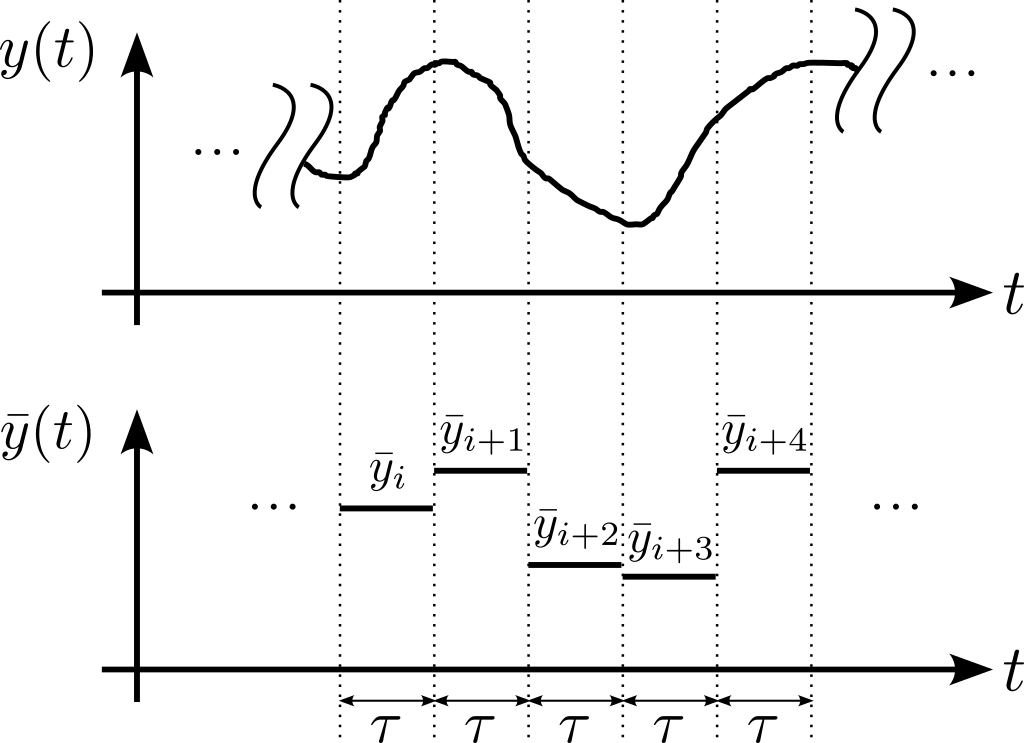
More concretely, suppose we have a continuous time series \(y(t)\, \), its Allan variance, \(\sigma^2_y(\tau)\, \), is defined as
\(\sigma^2_y(\tau) = \frac{1}{2} \langle ( \bar{y}_{i+1}\, – \bar{y}_{i} )^2 \rangle, \quad (1) \,\)
where \(\langle . \rangle \) denotes the expectation value (average) and \(\bar{y}_{i} \) is the ith sample of the average of y over observation time \(\tau \)(Figure 2). Allan deviation is then simply the square root of Allan variance, or \(\sigma(\tau) = \sqrt{\sigma^2(\tau)} \). One can evaluate this expression for a series of observation times \(\tau \) to gain insight into how self-similar (i.e., stable) the data is over different timescales.
As can be inferred from equation (1), the dimension of \(\sigma(\tau) \) matches that of y. We interpret the value to be the expected root mean square difference between two \(\tau\)-second-long measurements of y taken \(\tau \) seconds apart.
For example, consider a clock oscillating at \(f_0 = 50\,\text{MHz} \). If the Allan variance of its fractional frequency difference, Y, defined as
\(Y = \frac{f-f_0}{f_0} = \frac{\Delta f}{f_0}, \quad (2) \)
is \(1.23\times10^{-10} \) for a 10-second observation (\(\tau = 10\,\text{s} \)), then we would expect that two randomly chosen, consecutive, 10-second measurements of Y would differ by \(1.23\times10^{-10}\) RMS. Given the definition of fractional frequency difference, this is equivalent to an expected absolute frequency difference of \(\Delta f = 6.15\,\text{mHz} \) RMS.
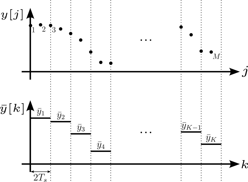
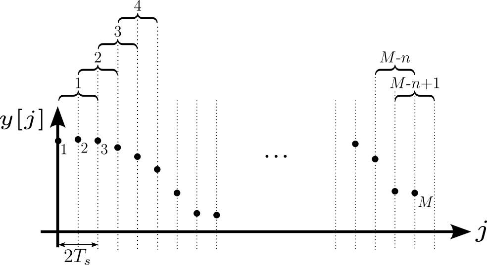
Consider now the case of a real, finite, dataset of length M, sampled with period \(T_s\, \) (Figure 3). In a sampled system we cannot choose the total time τ freely, so we divide the set into K segments of length \(\tau = n T_s\, \) for some \(n \in \mathbb{N}^+ \, \). The Allan variance may be approximated as
\(\sigma^2_y(\tau = nT_s) \simeq \frac{1}{2(K-1)} \sum_{i=1}^{K-1} (\bar{y}_{i+1}\, – \bar{y}_{i})^2. \quad (3) \,\)
Very roughly, the uncertainty in \(\sigma(\tau)\, \) is \(\pm \sigma(\tau)/\sqrt{K}\, \). A full treatment of measurement uncertainty is beyond the scope of this work, so see Ref [4] for more detail. To improve confidence in the results, and make more efficient use of valuable data, one can partition the data into overlapping segments (Figure 4). This yields \(M-2n+1 \,\) pairs of consecutive segments, as opposed to \(K-1=M/n-1 \,\) previously. This overlapping Allan deviation is given by
\(\sigma^2_y(\tau = nT_s) \simeq \frac{1}{2(M-2n+1)} \sum_{i=1}^{M-2n+1} (\bar{y}_{i+1}\, – \bar{y}_{i})^2. \quad (4) \,\)
Obtaining Allan variance via integration
In many common measurement scenarios, there exists a quantity x with the property that
\(x(t) = \int_0^t\, y(t’)\, {\rm d}t’\, . \quad (5)\,\)
For example, in clock stability measurements, where the time deviation, X, is the integral of the fractional frequency difference, Y, and in gyroscope systems where the measured angle, θ, is the integral of the rotation rate, Ω, i.e.
\(X(t) = \int_0^t\, Y(t’)\, {\rm d}t’\ \text{ and }\ \theta(t) = \int_0^t\, \Omega(t’)\, {\rm d}t’\, . \quad (6)\,\)
We are also free to compute x via numerical integration of equation (5), even if it does not correspond to a measured physical variable.
In such cases
\(\bar{y}(t) := \frac{1}{\tau}\int_t^{t+\tau}y(t’)\, {\rm d}t’ \quad (7) \,\)
\(= \frac{1}{\tau} [x(t+\tau) – x(t) ], \quad (8) \,\)
or in discrete terms,
\(\bar{y}_i = \frac{1}{\tau} [ x_{i+n} – x_i ] , \quad (9) \,\)
and equation (4) becomes
\(\sigma^2_y(\tau = nT_s) \simeq \frac{1}{2(nT_s^2)(N-2n)} \sum_{i=1}^{N-2n} (x_{i+2n} – 2x_{i+1}\, + x_{i})^2, \quad (10)\,\)
where N = M + 1 is the length of x. To understand this, consider that y may be constructed via numerical derivatives (differences) of x, so M = N − 1.
This may seem like an abstract simplification but for reasons of computational efficiency, Equation (10) provides the most commonly implemented formulation of Allan variance. Note that, here, measurements of x provide the Allan variance of y, not x.
Plotting Allan variance
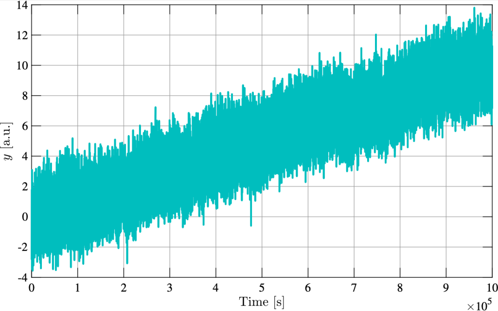
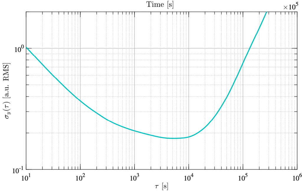
Allan variance is typically calculated for multiple averaging times and plotted on a log-log scale (Figure 5). Such plots are helpful in determining the best averaging time for a given measurement. Note that longer averaging times are not always preferable, particularly in the presence of low-frequency drifts.
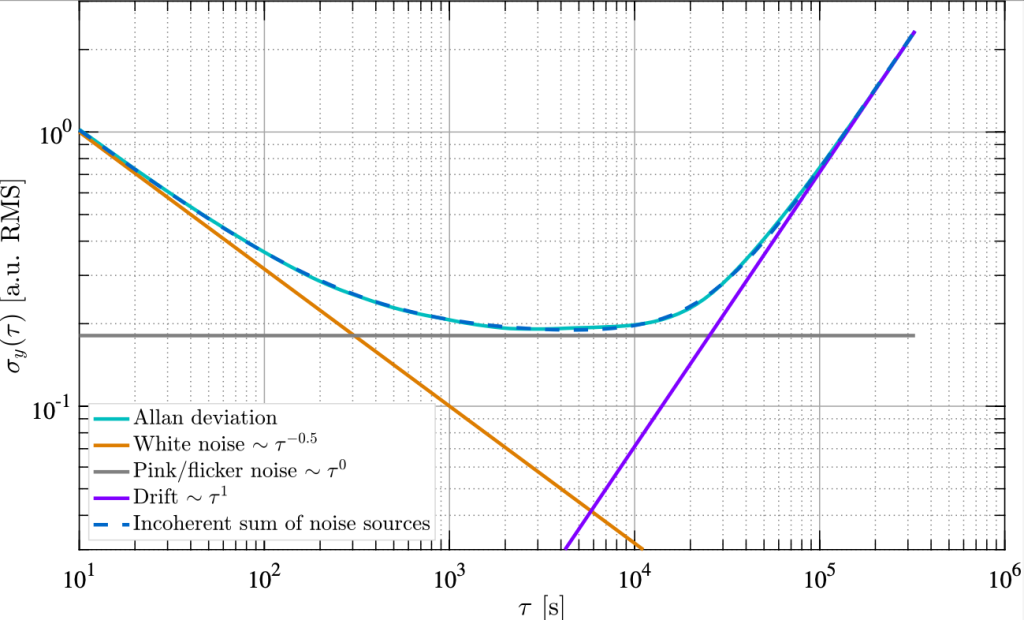
In addition, common noise sources are typically described by power laws, which present known slopes on Allan deviation plots. For example, white noise is reduced with the square root of averaging time. We would thus expect the slope of white noise to be \(\sigma_{\text{white}}(\tau) \sim 1/ \sqrt{\tau} \,\), and this is indeed the case. More generally, if the slope of a particular noise source in terms of power spectral density S is \(f^\alpha \,\), then the slope in terms of Allan deviation will be \(\tau^{-(\alpha+1)/2} \,\) . i.e.
\(S_y(f) \sim f^\alpha \Rightarrow \sigma(\tau) \sim \tau^{-(\alpha+1)/2}. \quad (11) \,\)
This fact allows one to easily determine which noise source is dominant over different averaging times, build a noise budget to ascertain whether system performance is well-understood, or quantify the contribution of each error source (Figure 6).
Table 1 presents the slopes of noise sources commonly encountered in the study of clocks and gyroscopes.
Table 1: Slope powers of \(\sigma(\tau)\,\) (i.e., β where \(\sigma(\tau) \sim \tau^\beta \,\)) for various noise sources in selected applications [3, 5]. FM: frequency modulation, PM: phase modulation.

Power spectral density vs. Allan variance
As mentioned, there are a number of tools available to describe the stability of a system. While Allan deviation is a time-domain metric of stability, a frequency-domain counterpart is the power spectral density (PSD), \(S_y\). If the dimension of y is \([u] \) then the dimension of \(S_y\) is \([u_{RMS}^2 / \text{Hz}] \). Of course, the information contained in the Allan deviation, \(\sigma_y(\tau) \), is simply an alternative representation of that contained in the PSD, and there exists a closed form conversion (see App. I of [6]). Note that it is only possible to convert from PSD to Allan variance and not the other way around. The conversion formula is:
\(\sigma_y^2(\tau) = \int_0^\infty S_y(f)\, |H(f)|^2\, {\rm d}f = 2 \int_0^\infty S_y(f) \left [\frac{\sin^4{(\pi\tau f)}}{(\pi \tau f)^2} \right ] {\rm d}f. \quad (12) \)
Here, \(H(f) \) is the transfer function of the time domain sampling function.
In this context, a useful expression to be aware of is
\(S_{y’}(f)=(2 \pi f)^2 S_y(f), \quad (13) \)
where \(y’ = \partial y / \partial t \). As an illustrative example, one may convert a PSD of phase (\phi) noise into one of frequency (f) noise according to \(S_{f}(f)= f^2 S_\phi (f). \)
Beyond Allan variance
Just as limitations were found with standard deviation, Allan deviation, too, is not the ideal statistic in all cases. Two commonly used derivatives of Allan deviation, offering improved performance in certain circumstances, are briefly discussed here for completeness.
Modified Allan deviation
We noted above the possibility of identifying noise sources based on the gradient traced on a plot of Allan deviation (Figure 6). Yet multiple noise sources present identical slopes. In particular, oscillator white phase modulation (WPM) noise and flicker phase modulation (FPM) noise both generate a slope of \(\tau^{-1} \) (see Table 1). However, WPM is sensitive to measurement bandwidth whereas FPM is not. By implementing an additional averaging over n adjacent measurements, where \(\tau = nT_s \), this modified Allan deviation, \(\rm{mod}\sigma_y(\tau)\), yields an effective bandwidth that narrows linearly with \(\tau \) and enables these noise sources to be differentiated [7]. The modified Allan variance is given by
\(\rm{mod}\, \sigma_y^2(\tau=nT_s) = \frac{1}{2} \left\langle \left [\frac{1}{n} \sum_{i=1}^n \left (\bar{y}_{i+n} – \bar{y}_i \right ) \right ]^2 \right\rangle, \quad (14)\)
or, more practically,
\(\rm{mod}\, \sigma^2_y(\tau = nT_s) \simeq \frac{1}{2n^2(nT_s)^2(N-3n+1)} \sum_{j=1}^{N-3n+1} \left [ \sum_{i=j}^{j+n-1} (x_{i+2n} – 2x_{i+1}\, + x_{i})\right ]^2, \quad (15)\)
with \(n \in \{1,2,…,N/3 \}. \)
Time deviation
A further metric, based on the modified Allan deviation, is the time deviation, or time Allan deviation \(TDEV(\tau) \), defined by
\(TDEV^2(\tau) = \frac{\tau^2}{3} \rm{mod}\, \sigma_y^2(\tau). \quad (16) \)
Note that this is nothing other than a “tilted” version of the modified Allan deviation (all slopes on a log-log plot will be reduced by one power of \(\tau \)). The normalization factor is chosen such that \(TDEV(\tau)\) agrees with the standard deviation for white phase modulation (WPM) noise when \(n = 1\).
TDEV is also often denoted by \(\sigma_x(\tau)\), making explicit the fact that it describes the stability of x (rather than y), due to the additional factor of \(\tau \).
As the name suggests, this measure is useful in the characterization of distributed timing signals, where it is used to describe the phase variation of a clock as a function of averaging time.
Allan deviation with the Moku:Delta Phasemeter
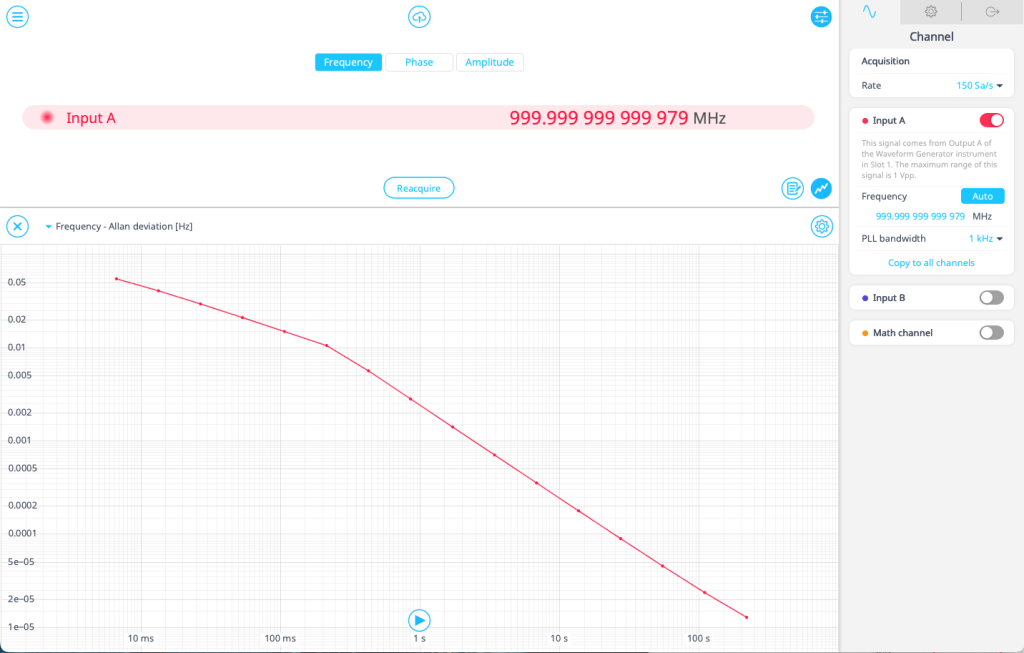
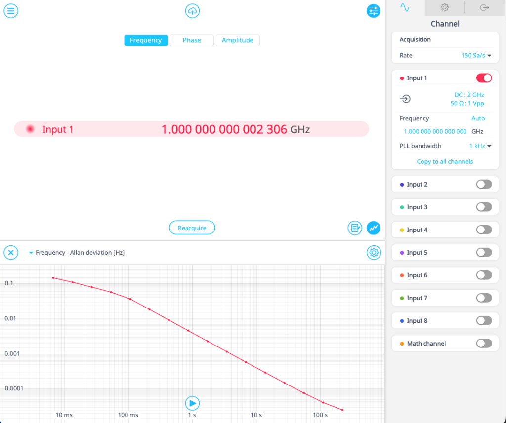
In this example, we measure the Allan deviation of a 1 GHz signal with Moku:Delta Phasemeter. An external microwave synthesizer generates a 1 GHz tone which is fed into the Delta analog front end. Launching the Phasemeter instrument on Delta, we can see the measured frequency, phase, and amplitude of the signal. Under Input 1, we set the frequency to 1 GHz and the PLL bandwidth to 1 kHz. We click the button to display the plot in real time and, under the drop-down menu, select “Frequency – Allan deviation [Hz].” We refresh the measurement by clicking “Reacquire” and watch the plot populate for around 15 minutes. The results, calculated using equation (10), are shown in Figure 7.
Conclusion
In this work we have provided an introduction to Allan variance, demonstrating how it may be computed and interpreted. Originally developed in the context of oscillator stability, this is still where the statistic is most often employed. However, we emphasize that it is applicable to any time series and useful in a broad range of fields.
Allan variance can assist in both determining the ideal observation time for a particular measurement and identifying dominant noise sources. Conversion from power spectral densities to Allan variance is also possible.
Allan variance is a valuable statistical tool, and is one of many such tools available for data post-processing on the Moku Phasemeter. This capability, along with the Phasemeter’s microradian accuracy and intuitive interface via the Moku app, make Moku an exceptional device for characterizing the stability of oscillator systems.
References
[1] D. W. Allan, “Statistics of atomic frequency standards,” IEEE Proceedings, vol. 54, pp. 221–230, Feb. 1966.
[2] L. Hua, Y. Zhuang, L. Qi, J. Yang, and L. Shi, “Noise Analysis and Modeling in Visible Light Communication Using Allan Variance,” IEEE Access, vol. 6, pp. 74 320–74 327, 2018.
[3] IEEE, “IEEE Standard Specification Format Guide and Test Procedure for Single-Axis Interferometric Fiber Optic Gyros,” IEEE Std 952-1997, pp. 1–84, 1997.
[4] C. A. Greenhall and W. Riley, “Uncertainty of Stability Variances Based on Finite Differences,” September 2004. [Online]. Available: https://ntrs.nasa.gov/citations/20050061319
[5] W. Riley and D. Howe, “NIST Special Publication 1065: Handbook of Frequency Stability Analysis,” July 2008. [Online]. Available: https://tsapps.nist.gov/publication/getpdf.cfm?pub id=50505
[6] J. A. Barnes, A. R. Chi, L. S. Cutler, D. J. Healey, D. B. Leeson, T. E. McGunigal, J. A. Mullen, W. L. Smith, R. L. Sydnor, R. F. C. Vessot, and G. M. R. Winkler, “Characterization of frequency stability,” IEEE Transactions on Instrumentation and Measurement, vol. IM-20, no. 2, pp. 105–120, 1971.
[7] D. W. Allan and J. A. Barnes, “A Modified “Allan Variance” with In- creased Oscillator Characterization Ability,” in Proc. 35th Ann. Freq. Control Symposium. USAERADCOM, Ft. Nonmouth, NJ 07703: Time and Frequency Division, National Bureau of Standards, May 1981, https://tf.nist.gov/general/pdf/560.pdf.


